uwot is the a package for implementing the UMAP
dimensionality reduction method. For more information on UMAP, see the
original paper and the Python package.
We’ll use the iris dataset in these examples. It’s not
the ideal dataset because it’s not terribly large nor high-dimensional
(with only 4 numeric columns), but you’ll get the general idea.
The default output dimensionality of UMAP is into two-dimensions, so
it’s amenable for visualization, but you can set a larger value with
n_components. In this vignette we’ll stick with two
dimensions. We will need a function to make plotting easier:
kabsch <- function(pm, qm) {
  pm_dims <- dim(pm)
  if (!all(dim(qm) == pm_dims)) {
    stop(call. = TRUE, "Point sets must have the same dimensions")
  }
  # The rotation matrix will have (ncol - 1) leading ones in the diagonal
  diag_ones <- rep(1, pm_dims[2] - 1)

  # center the points
  pm <- scale(pm, center = TRUE, scale = FALSE)
  qm <- scale(qm, center = TRUE, scale = FALSE)

  am <- crossprod(pm, qm)

  svd_res <- svd(am)
  # use the sign of the determinant to ensure a right-hand coordinate system
  d <- determinant(tcrossprod(svd_res$v, svd_res$u))$sign
  dm <- diag(c(diag_ones, d))

  # rotation matrix
  um <- svd_res$v %*% tcrossprod(dm, svd_res$u)

  # Rotate and then translate to the original centroid location of qm
  sweep(t(tcrossprod(um, pm)), 2, -attr(qm, "scaled:center"))
}
iris_pca2 <- prcomp(iris[, 1:4])$x[, 1:2]
plot_umap <- function(coords, col = iris$Species, pca = iris_pca2) {
  plot(kabsch(coords, pca), col = col, xlab = "", ylab = "")
}
Most of this code is just the kabsch
algorithm to align two point sets, which I am going to use to align
the results of UMAP over the first two principal components. This is to
keep the relative orientation of the output the same across different
plots which makes it a bit easier to see the differences between them.
UMAP is a stochastic algorithm so the output will be different each time
you run it and small changes to the parameters can affect the
absolute values of the coordinates, although the interpoint
differences are usually similar. There’s no need to go to such trouble
in most circumstances: the output of umap is a perfectly
useful 2D matrix of coordinates you can pass into a plotting function
with no further processing required.
Basic UMAP
The defaults of the umap function should work for most
datasets. No scaling of the input data is done, but non-numeric columns
are ignored:

Parameters
uwot has accumulated many parameters over time, but most
of the time there are only a handful you need worry about. The most
important ones are:
min_dist
This is a mainly aesthetic parameter, which defines how close points
can get in the output space. A smaller value tends to make any clusters
in the output more compact. You should experiment with values between 0
and 1, although don’t choose exactly zero. The default is 0.01, which
seems like it’s a bit small for iris. Let’s crank up
min_dist to 0.3:
This has made the clusters bigger and closer together, so we’ll use
min_dist = 0.3 for the other examples with
iris.
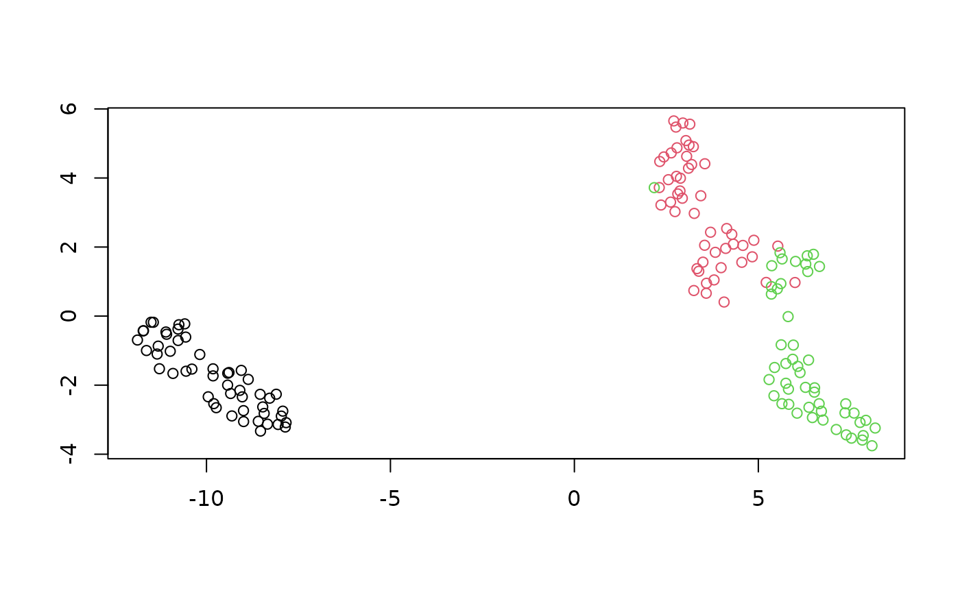
n_neighbors
This defines the number of items in the dataset that define the neighborhood around each point. Set it too low and you will get a more fragmented layout. Set it too high and you will get something that will miss a lot of local structure.
Here’s a result with 5 neighbors:
set.seed(42)
iris_umap_nbrs5 <- umap(iris, n_neighbors = 5, min_dist = 0.3)
plot_umap(iris_umap_nbrs5)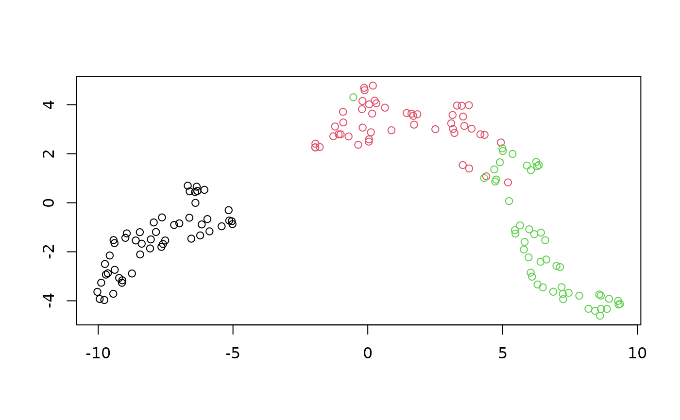
It’s not hugely different from the default of 15 neighbors, but the clusters are a bit more broken up.
There should be a more pronounced difference going the other way and looking at 100 neighbors:
set.seed(42)
iris_umap_nbrs100 <- umap(iris, n_neighbors = 100, min_dist = 0.3)
plot_umap(iris_umap_nbrs100)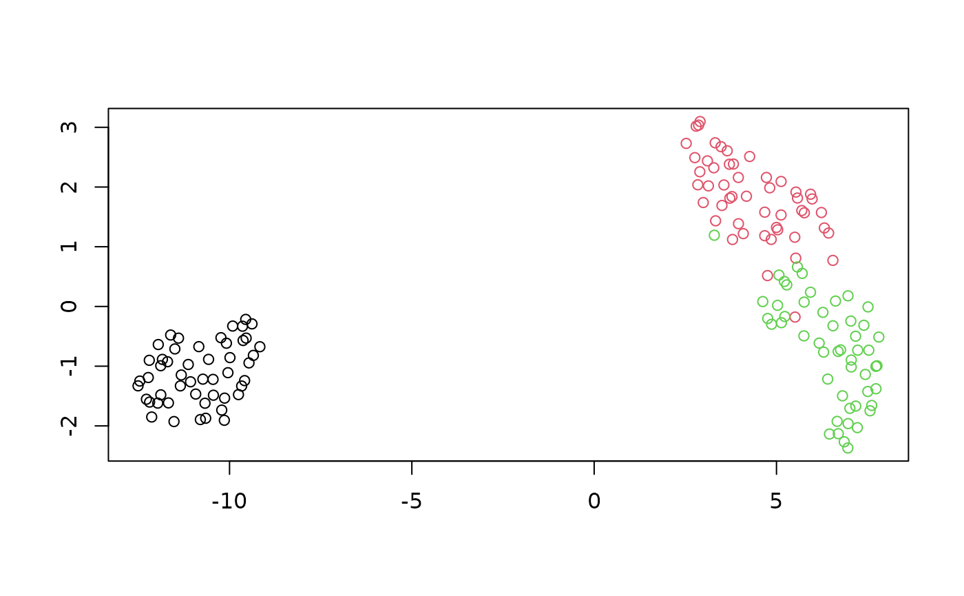
Here there is a much more uniform appearance to the results. It’s
always worth trying a few different values of n_neighbors,
especially larger values, although larger values of
n_neighbors will lead to longer run times. Sometimes small
clusters that you think are meaningful may in fact be artifacts of
setting n_neighbors too small, so starting with a larger
value and looking at the effect of reducing n_neighbors can
help you avoid over interpreting results.
init
The default initialization of UMAP is to use spectral initialization,
which acts upon the (symmetrized) k-nearest neighbor graph that is in
determined by your choice of n_neighbors. This is usually a
good choice, but it involves a very sparse matrix, which can sometimes
be a bit too sparse, which leads to numerical difficulties
which manifest as slow run times or even hanging calculations. If your
dataset causes these issues, you can either try increasing
n_neighbors but I have seen cases where that would be
inconvenient in terms of CPU and RAM usage. An alternative is to use the
first two principal components of the data, which at least uses the data
you provide to give a solid global picture of the data that UMAP can
refine. It’s not appropriate for every dataset, but in most cases, it’s
a perfectly good alternative.
The only gotcha with it is that depending on the scaling of your
data, the initial coordinates can have large inter-point distances. UMAP
will not optimize that well, so such an output should be scaled to a
small standard deviation. If you set init = "spca", it will
do all that for you, although to be more aligned with the UMAP
coordinate initialization, I recommend you also set
init_sdev = "range" as well. init_sdev can
also take a numerical value for the standard deviation. Values from
1e-4 to 10 are reasonable, but I recommend you
stick to the default of "range".
set.seed(42)
iris_umap_spca <-
  umap(iris,
    init = "spca",
    init_sdev = "range",
    min_dist = 0.3
  )
plot_umap(iris_umap_spca)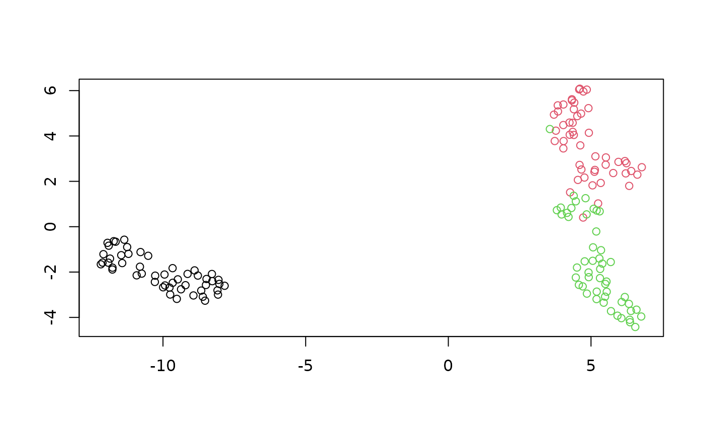
This doesn’t have a big effect on iris, but it’s good to
know about this as an option: and it can also smooth out the effect of
changing n_neighbors on the initial coordinates with the
standard spectral initialization, which can make it easier to see the
effect of changing n_neighbors on the final result.
Some other init options to know about:
-
"random": if the worst comes to the worst, you can always fall back to randomly assigning the initial coordinates. You really want to avoid this if you can though, because it will take longer to optimize the coordinates to the same quality, so you will need to increasen_epochsto compensate. Even if you do that, it’s much more likely that you will end up in a minimum that is less desirable than one based on a good initialization. This will make interpreting the results harder, as you are more likely to end up with different clusters beings split or mixed with each other. - If you have some coordinates you like from another method, you can
pass them in as a matrix. But remember will probably want to scale them
with
init_sdevthough.
dens_scale
The dens_scale parameter varies from 0 to 1 and controls
how much of the relative densities of the input data is attempted to be
preserved in the output.
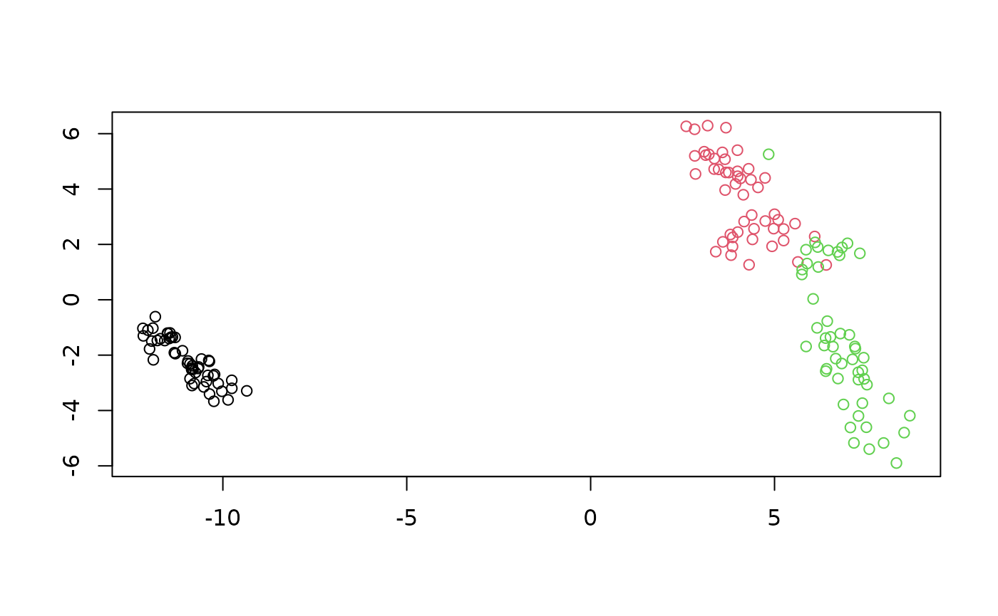
This has shrunk the black cluster on the left of the plot (those are
of species setosa), which reflect that the density of the
setosa points is less spread out in the input data than the
other two species. For more on dens_scale please read its
dedicated article.
Embedding New Data
Once you have an embedding, you can use it to embed new data,
although you need to remember to ask for a “model” to return. Instead of
just the coordinates, you will now get back a list which contains all
the extra parameters you will need for transforming new data. The
coordinates are still available in the $embedding
component.
Let’s try building a UMAP with just the setosa and
versicolor iris species:
set.seed(42)

iris_train <- iris[iris$Species %in% c("setosa", "versicolor"), ]
iris_train_umap <-
  umap(iris_train, min_dist = 0.3, ret_model = TRUE)
plot(
  iris_train_umap$embedding,
  col = iris_train$Species,
  xlab = "",
  ylab = "",
  main = "UMAP setosa + versicolor"
)
Next, you can use umap_transform to embed the new
points:
iris_test <- iris[iris$Species == "virginica", ]
set.seed(42)
iris_test_umap <- umap_transform(iris_test, iris_train_umap)
plot(
  rbind(iris_train_umap$embedding, iris_test_umap),
  col = iris$Species,
  xlab = "",
  ylab = "",
  main = "UMAP transform virginica"
)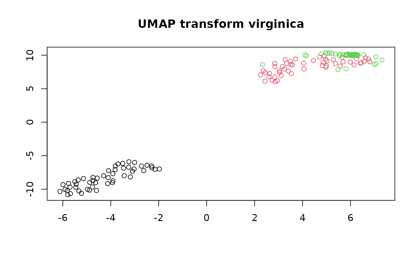
The green points in the top-right show the embedded data. Note that
the original (black and red) clusters do not get optimized any further.
While we haven’t perfectly reproduced the full UMAP, the
virginica points are located in more or less the right
place, close to the versicolor items. Just like with any
machine learning method, you must be careful with how you choose your
training set.
Supported Distances
For small (N < 4096) and Euclidean distance, exact nearest
neighbors are found using the FNN package.
Otherwise, approximate nearest neighbors are found using RcppAnnoy. The
supported distance metrics (set by the metric parameter)
are:
- Euclidean
- Cosine
- Pearson Correlation (
correlation) - Manhattan
- Hamming
Exactly what constitutes the cosine distance can differ between
packages. uwot tries to follow how the Python version of
UMAP defines it, which is 1 minus the cosine similarity. This differs
slightly from how Annoy defines its angular distance, so be aware that
uwot internally converts the Annoy version of the distance.
Also be aware that the Pearson correlation distance is the cosine
distance applied to row-centered vectors.
If you need other metrics, and can generate the nearest neighbor info
externally, you can pass the data directly to uwot via the
nn_method parameter. Please note that the Hamming support
is a lot slower than the other metrics. I do not recommend using it if
you have more than a few hundred features, and even then expect it to
take several minutes during the index building phase in situations where
the Euclidean metric would take only a few seconds.
Multi-threading support
Parallelization can be used for the nearest neighbor index search, the smooth knn/perplexity calibration, and the optimization, which is the same approach that LargeVis takes.
You can (and should) adjust the number of threads via the
n_threads, which controls the nearest neighbor and smooth
knn calibration, and the n_sgd_threads parameter, which
controls the number of threads used during optimization. For the
n_threads, the default is the number of available cores.
For n_sgd_threads the default is 0, which
ensures reproducibility of results with a fixed seed.
Python Comparison
For the datasets I’ve tried it with, the results look at least
reminiscent of those obtained using the official Python
implementation. Below are results for the 70,000 MNIST digits
(downloaded using the snedata package).
Below, is the result of using the official Python UMAP implementation
(via the reticulate
package). Under that is the result of using uwot.
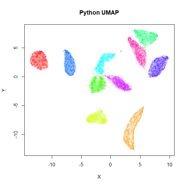
MNIST UMAP (Python)
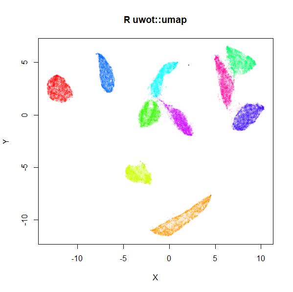
MNIST UMAP (R)
The project documentation contains some more examples, and comparison with Python.
Limitations and Other Issues
Nearest Neighbor Calculation
uwot leans heavily on the Annoy library for
approximate nearest neighbor search. As a result, compared to the Python
version of UMAP, uwot has much more limited support for
different distance measurements, and no support for sparse matrix data
input.
However, uwot does let you pass in nearest
neighbor data. So if you have access to other nearest neighbor methods,
you can generate data that can be used with uwot. See the
Nearest
Neighbor Data Format article. Or if you can calculate a distance
matrix for your data, you can pass it in as dist
object.
For larger distance matrices, you can pass in a
sparseMatrix (from the Matrix
package).
Experience with COIL-100,
which has 49,152 features, suggests that Annoy will definitely
struggle with datasets of this dimensionality. Even 3000 dimensions can
cause problems, although this is not a difficulty specific to Annoy.
Reducing the dimensionality with PCA to an intermediate dimensionality
(e.g. 100) can help. Use e.g. pca = 100 to do this. This
can also be slow on platforms without good linear algebra support and
you should assure yourself that 100 principal components won’t be
throwing away excessive amounts of information.
Spectral Initialization
The spectral initialization default for umap (and the
Laplacian Eigenmap initialization, init = "laplacian") can
sometimes run into problems. If it fails to converge it will fall back
to random initialization, but on occasion I’ve seen it take an extremely
long time (a couple of hours) to converge. Recent changes have hopefully
reduced the chance of this happening, but if initialization is taking
more than a few minutes, I suggest stopping the calculation and using
the scaled PCA (init = "spca") instead.
Supporting Libraries
All credit to the following packages which do a lot of the hard work:
- Coordinate initialization uses RSpectra to do the eigendecomposition of the normalized Laplacian.
- The optional PCA initialization and initial dimensionality reduction uses irlba.
- The smooth k-nearest neighbor distance and stochastic gradient descent optimization routines are written in C++ (using Rcpp, aping the Python code as closely as possible.
- Some of the multi-threading code is based on RcppParallel.