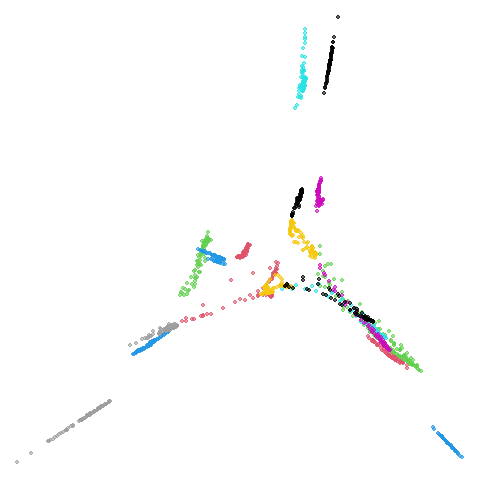
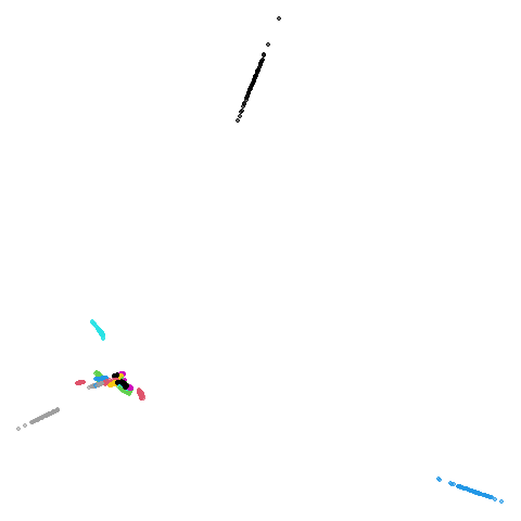
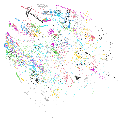
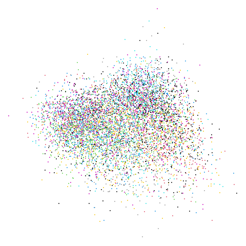
Mid-Spectral Initialization
December 31 2024
Source:vignettes/articles/mid-spectral-initialization.Rmd
mid-spectral-initialization.RmdIntroduction
The initialization
article describes some ways to initialize the embedding process.
Really you have two options: a spectral initialization (the default) and
PCA, which is what you will use if the affinity graph contains
disconnected components. A third option, the “approximate global”
spectral method attempts to allow for spectral initialization in the
face of disconnections by adding some random edges to the affinity
graph. This mainly works, but it did change the results for the
isoswiss dataset (and not for the better) suggesting that
the agspectral initialization was perturbing the
coordinates in a way that was not helpful.
One of the things that PaCMAP does is include the concept of “mid-near” pairs. The process is:
- Pick
nrandom neighbors for each point (nis usually 6) - Sort them by distance and keep the
k-th closest (kis usually 2) - Repeat
mtimes (mis usually 10).
This results in each point having m neighbors where the
distribution isn’t uniformly random, but is instead biased towards
slightly nearer neighbors.
In PaCMAP, these are added to the graph as additional edges, but given a different set of weights and schedule in the first phases of the optimization.
Because they are not involved in the final step of the optimization, you could view the mid-near pairs as a way of enforcing extra longer-range structure for the final stage of the embedding fine-tunes the layout. So could we add these to the spectral initialization and get some extra structure in the initial embedding? At the very least, it’s likely that adding these extra edges will help with the disconnected components problem and allow for a spectral-like initialization.
Implementation
Here’s how I imagine this working:
- Create the mid-near pairs as described above.
- Use the
uwotfunctionsimilarity_graphto generate a “mid affinity graph” using the mid-near pairs. - Create the nearest neighbor graph in the usual way. You can also use
similarity_graphfor this. - Combine the two graphs by adding the mid-near pairs to the nearest neighbor graph. Probably we will need to ensure the emphasis remains on the nearest neighbor graph, so this should be a weighted sum of the two graphs.
- Do spectral initialization on the combined graph.
- Use this as the initial embedding for the optimization.
Below are some functions to make this work. Note that:
- You need to have rnndescent installed.
- You will need to borrow the
sort_knn_graphfunction from the code given in the locally-scaled-neighbors article. - There are tons of internal
uwotfunctions used here. I do not plan to support this officially at the moment, but I don’t want to break this myself, so it’s likely to be stable (or I will update the code below to keep it working with future versions ofuwot). - In the code below I assume you have generated the nearest neighbors
externally to
uwotvia something likernndescent. Becausesimiliarity_graphcan return the nearest neighbors (viaret_extra = "nn") the code could be changed to allow for the nearest neighbors to be returned from callingmid_spectral_initdirectly. I leave this as an exercise for the reader. - I have also assumed we always use Euclidean distance.
rnndescent::random_knncan use other distances, but I have not implemented this here.
To use this code do something like:
nn_graph <- rnndescent::rnnd_knn(X, k = 15)
init_coords <- mid_spectral_init(X, nn_graph, mid_nnbrs = 4, graph_weight = 0.9)
umap_res <- umap2(X, nn_method = nn_graph, init = init_coords)
The two parameters you are most likely to want to play around with
are mid_nnbrs and graph_weight. The former is
the number of mid-near pairs to generate for each point, and the latter
is the weight to give the nearest neighbor graph in the combined graph.
The higher the value, the more like the typical spectral initialization
you will get.
pacmap_mid_nbrs <- function(X,
                            k = 10,
                            n_rand = 6,
                            nth_closest = 2,
                            ...) {
  varargs <- list(...)
  varargs$data <- Matrix::t(X)
  varargs$k <- n_rand
  varargs$obs <- "C"
  if (is.null(varargs$threads)) {
    varargs$n_threads <- default_num_threads()
  }

  res <- list(
    idx = matrix(0, nrow = nrow(X), ncol = k),
    dist = matrix(0.0, nrow = nrow(X), ncol = k)
  )

  for (i in 1:k) {
    random_nbrs <- do.call(rnndescent::random_knn, varargs)
    res$idx[, i] <- random_nbrs$idx[, nth_closest]
    res$dist[, i] <- random_nbrs$dist[, nth_closest]
  }
  res <- sort_knn_graph(res, enforce_self_first = FALSE)
  res
}

weighted_affinity_graph <- function(X,
                                    nn_graph,
                                    midn_graph = NULL,
                                    mid_nnbrs = 10,
                                    mid_select = 6,
                                    mid_nth_closest = 2,
                                    graph_weight = 0.9,
                                    n_threads = NULL,
                                    verbose = FALSE) {
  if (is.null(n_threads)) {
    n_threads <- default_num_threads()
  }
  if (is.null(midn_graph)) {
    if (is.null(X)) {
      stop("X must be provided if midn_graph is NULL")
    }
    uwot:::tsmessage(
      "Generating mid neighbor graph with mid_nnbrs=",
      mid_nnbrs,
      " (",
      mid_nth_closest,
      " from ",
      mid_select,
      ")",
      " using ",
      n_threads,
      " threads"
    )
    midn_graph <- pacmap_mid_nbrs(
      X,
      k = mid_nnbrs,
      n_rand = mid_select,
      nth_closest = mid_nth_closest,
      n_threads = n_threads
    )
  }

  uwot:::tsmessage("Generating near-affinity graph")
  nbr_affinity_graph <- uwot::similarity_graph(
    nn_method = nn_graph,
    n_threads = n_threads,
    verbose = FALSE
  )

  uwot:::tsmessage("Generating mid-affinity graph")
  mid_affinity_graph <- uwot::similarity_graph(
    nn_method = midn_graph,
    n_threads = n_threads,
    verbose = FALSE
  )

  uwot:::tsmessage(
    "Combining near and mid neighbor graphs with graph weight ",
    graph_weight
  )
  if (graph_weight == 1) {
    affinity_graph <- nbr_affinity_graph
  } else if (graph_weight == 0) {
    affinity_graph <- mid_affinity_graph
  } else {
    affinity_graph <- graph_weight * nbr_affinity_graph +
      (1 - graph_weight) * mid_affinity_graph
  }

  affinity_graph
}

mid_spectral_init <- function(X,
                              nn_graph,
                              midn_graph = NULL,
                              mid_nnbrs = 5,
                              mid_select = 6,
                              mid_nth_closest = 2,
                              graph_weight = 0.9,
                              n_threads = NULL,
                              verbose = FALSE) {
  if (is.null(n_threads)) {
    n_threads <- uwot:::default_num_threads()
  }

  affinity_graph <- weighted_affinity_graph(
    X = X,
    nn_graph = nn_graph,
    midn_graph = midn_graph,
    mid_nnbrs = mid_nnbrs,
    mid_select = mid_select,
    mid_nth_closest = mid_nth_closest,
    graph_weight = graph_weight,
    n_threads = n_threads,
    verbose = verbose
  )

  coords <- uwot:::spectral_init(affinity_graph, verbose = verbose)

  uwot:::tsmessage("Finished initializing")
  coords
}
Datasets
Brief descriptions of the datasets used here can be found in the examples article.
Effect of weight on initial coordinates
In the following I have set mid_nnbrs = 4. We don’t want
the number of these edges to be too high, because we shouldn’t need too
many to get a fully connected graph. In practice I have found that
mid_nnbrs = 2 is also fine, and usually
mid_nnbrs = 1 also works.
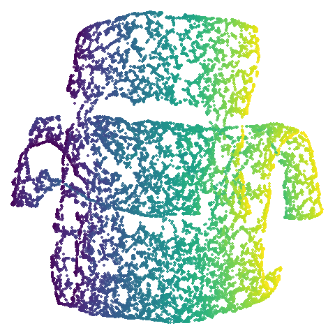
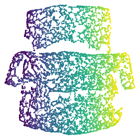
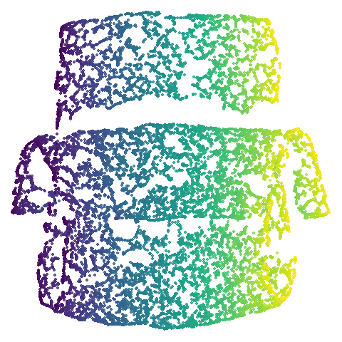
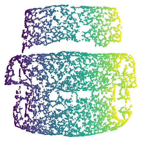
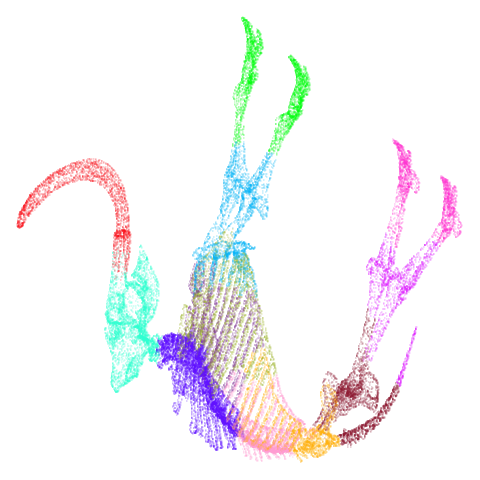
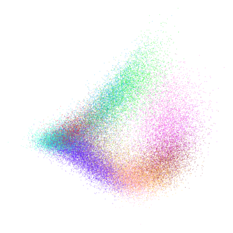
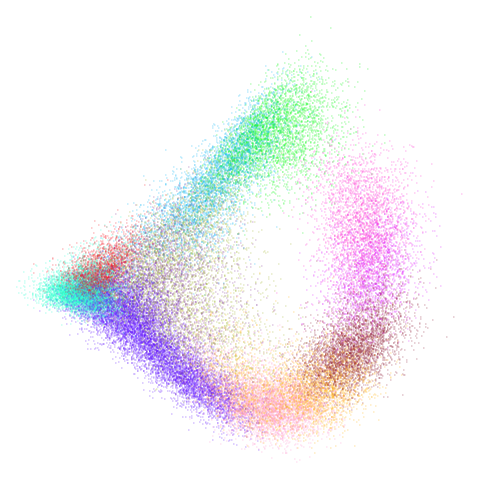
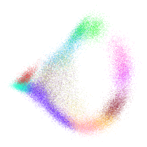
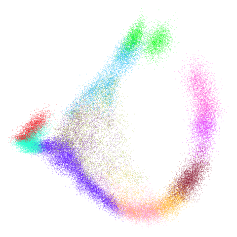
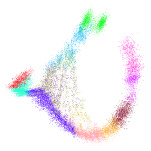
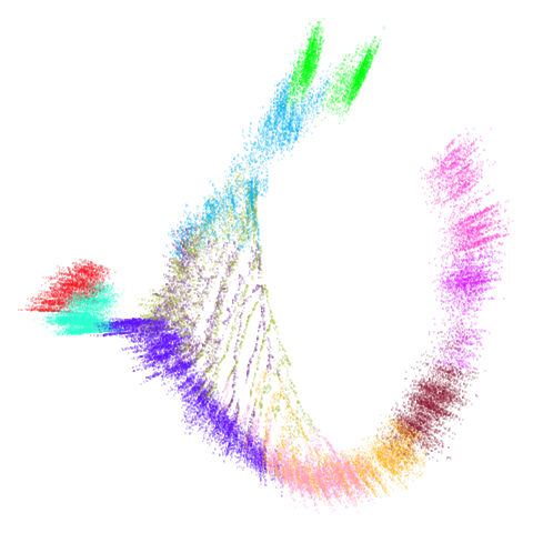
Let’s take a look at mammoth to start with. It has a
very different result if you initialize with the spectral method vs PCA.
Below are the initial mid-spectral initialization with different values
of graph_weight, which is given in the header of the table
cell. As we go left to right, top to bottom we increase from 0 (just use
mid-near neighbors) to 1 (only use k-nearest neighbors, standard
spectral initialization). I’ve also included the PCA results for
comparison.
mammoth
| pca | 0 | 0.25 |
|---|---|---|
 |
 |
 |
| 0.5 | 0.75 | 0.9 |
|---|---|---|
 |
 |
 |
| 0.99 | 0.999 | 1 |
|---|---|---|
 |
 |
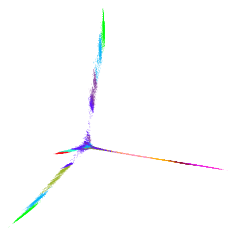 |
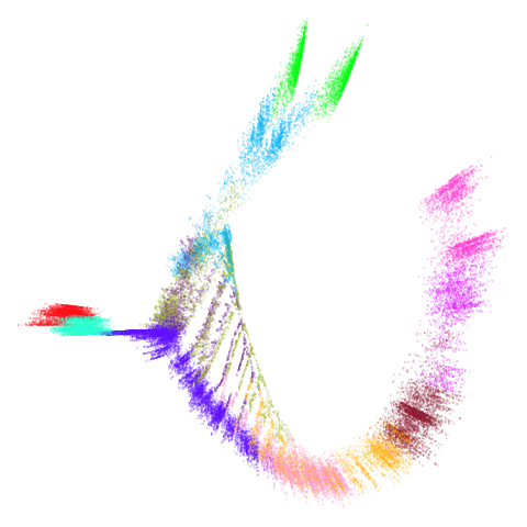
First of all, sorry about the odd orientation of the mammoth, but them’s the breaks. What’s apparent is that the addition of mid-near neighbors immediately makes the coordinates take on a very similar layout to the PCA initialization. Now I know you’re saying “no, it looks like a fuzzy mess”. True, but you can see that the legs are placed together, i.e. it’s the same side-on view as the PCA result. Compare that to the k-nearest neighbors initialization (bottom right), which is more like looking at the mammoth from above. There are two lines, one at about 12 o’clock and the other at about 7 o’clock. Those are the legs, clearly separate from each other, and split by the torso.
What’s more than slightly annoying to me is that I have been unable
to reproduce the “pure” spectral initialization with any value of
graph_weight < 1. The presence of the mid-near edges
pushes the coordinates into the “PCA-like” orientation. Now the good
news there is that the PaCMAP paper makes great hay of the mammoth
embedding looking more sensible under their method than UMAP and part of
that is the side-on view.
In terms of why this happens, it’s notable that the mammoth spectral
initialization takes a comparative age to converge. Most initializations
for datasets of this size (50,000 items) take a second, or a couple of
seconds at most. Spectral initialization chugs along for nearly a
minute. That’s not a good sign, so there must be something about the
mammoth dataset that makes it troublesome. Probably fiddling with the
parameters to RSpectra’s solution (more memory, more
iterations) would help, but the mid-spectral initialization is not
necessarily worse than the spectral initialization and it also completes
in a second.
isoswiss
Another low-dimensional dataset, but this one is the classic manifold
that is perfect for a spectral approach (well, apart from the repeated eigendirections
problem, but UMAP optimization helps fix that). What you certainly
won’t want to do is to use PCA in this case. Given that PCA-ness seems
to creep into the mammoth results with
graph_weight < 1, let’s see what happens.
| pca | 0 | 0.25 |
|---|---|---|
 |
 |
 |
| 0.5 | 0.75 | 0.9 |
|---|---|---|
 |
 |
 |
| 0.99 | 0.999 | 1 |
|---|---|---|
 |
 |
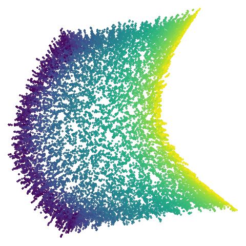 |
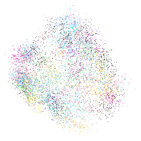
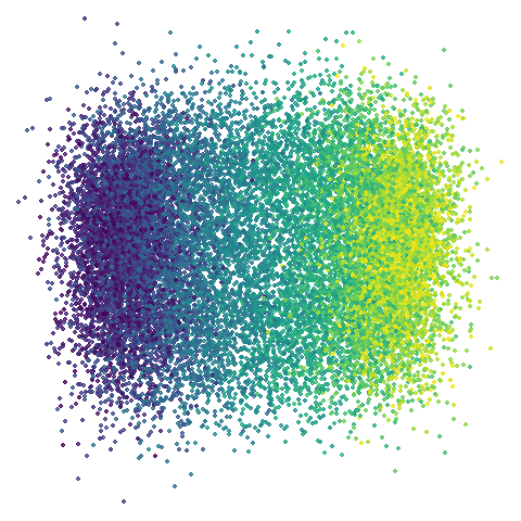
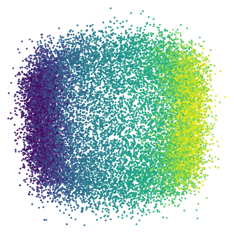
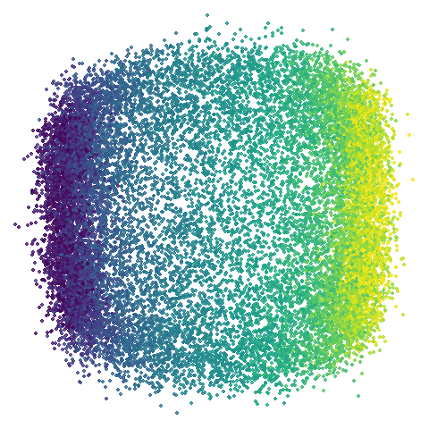
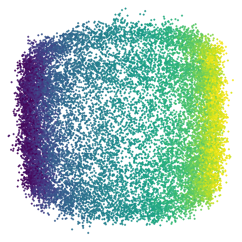
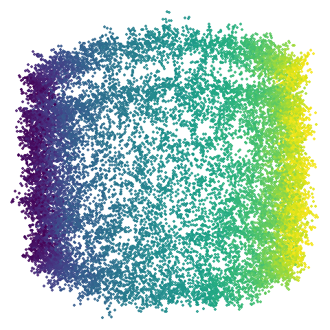
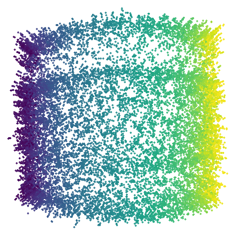
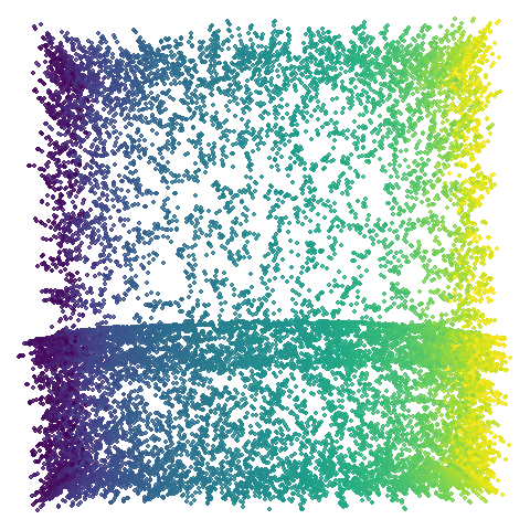
Hard to really see here, but in the pca case you are
basically looking at the swiss role perpendicular to rolled up part. So
those apparent four darker lines are where the folding is occurring. The
mid-spectral cases all struggle to avoid wanting to fold it up or just
make what seems like a bit of a mess. The closes we get is with
graph_weight = 0.999. If you increase the graph_weight to
0.9999 you do get the fully unrolled swiss roll,
but that doesn’t work for mammoth, and if you are up at the
four 9s you might as well just do the normal spectral initialization at
this point.
One more low-dimensional and manifold-based dataset:
scurvehole
| pca | 0 | 0.25 |
|---|---|---|
 |
 |
 |
| 0.5 | 0.75 | 0.9 |
|---|---|---|
 |
 |
 |
| 0.99 | 0.999 | 1 |
|---|---|---|
 |
 |
 |
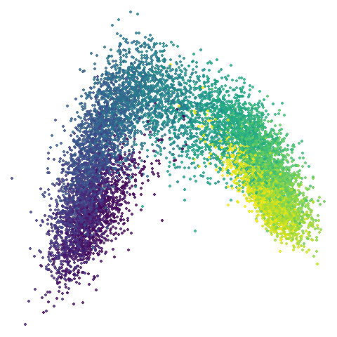
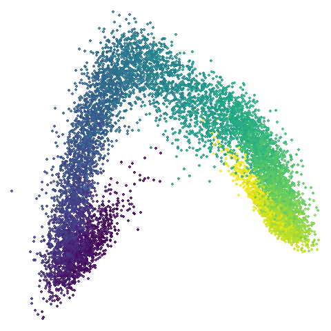
No real sign of the PCA result here. The “horseshoe” shape is
apparent at most settings. On the one hand that is characteristic of the
spectral initialization. On the other, this is a classic sign of the
“repeated eigendirections problem”, but we aren’t going to solve that
here. You do have to get all the way to
graph_weight = 0.999 to get weird hook-looking appendages
at the end of the curve to disappear, but at least we get there.
I don’t really care about these datasets. Let’s take a look at a
higher dimensional more “blobby” dataset. Like mnist:
mnist
| pca | 0 | 0.25 |
|---|---|---|
 |
 |
 |
| 0.5 | 0.75 | 0.9 |
|---|---|---|
 |
 |
 |
| 0.99 | 0.999 | 1 |
|---|---|---|
 |
 |
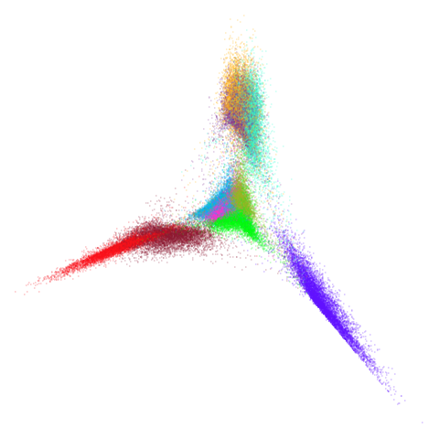 |
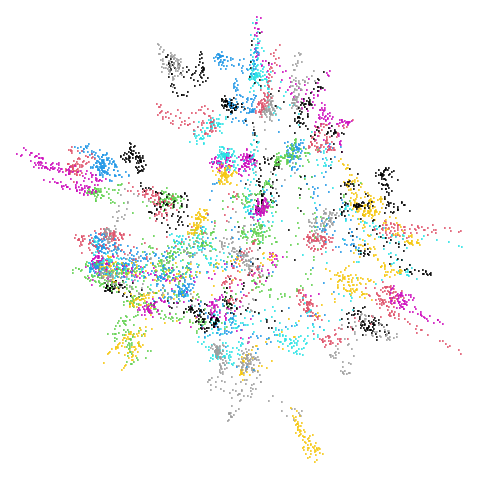
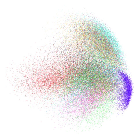
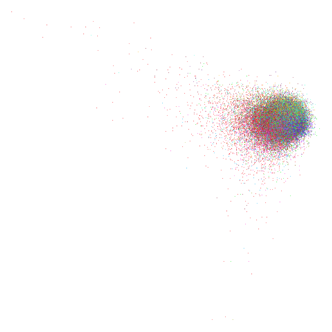
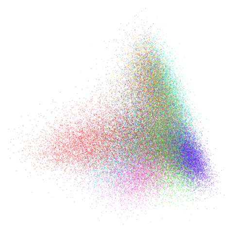
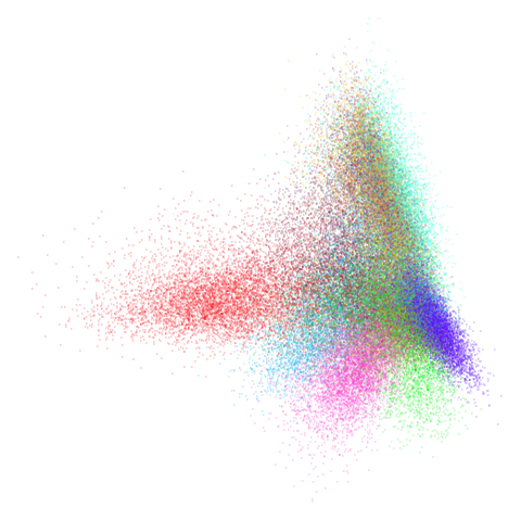
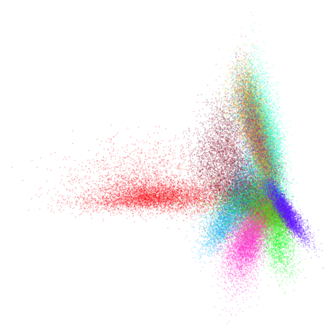
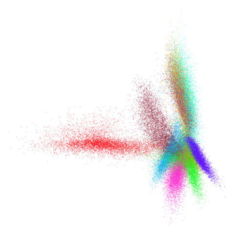
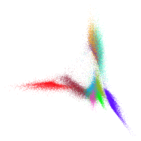
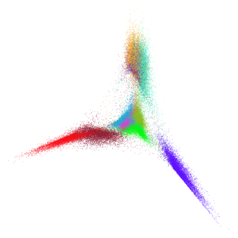
You can also get to something that looks very spectral-like with with
a graph_weight = 0.99 or above. And the
graph_weight = 0.9 results is quite pleasing, showing a
visible cluster structure and seeming to sit intermediate between the
PCA and spectral result. That’s more like it.
Let’s try one more high-dimensional dataset:
fashion
| pca | 0 | 0.25 |
|---|---|---|
 |
 |
 |
| 0.5 | 0.75 | 0.9 |
|---|---|---|
 |
 |
 |
| 0.99 | 0.999 | 1 |
|---|---|---|
 |
 |
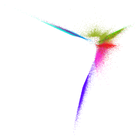 |
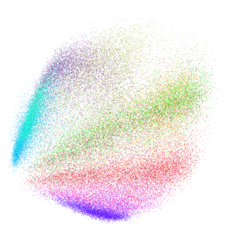
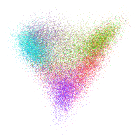
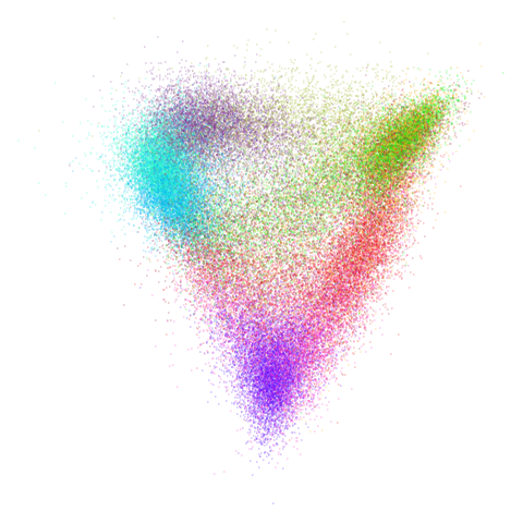
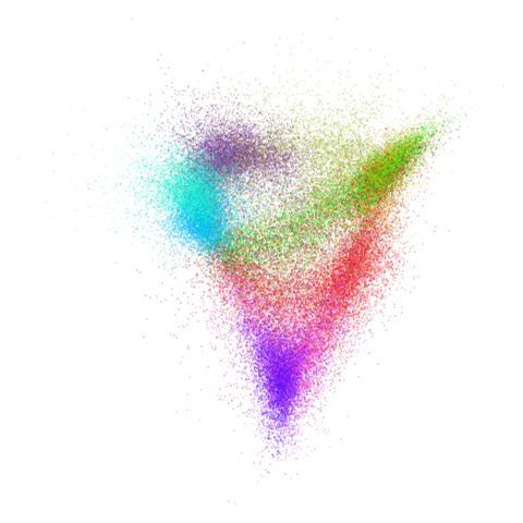
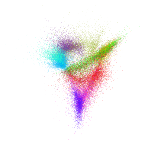
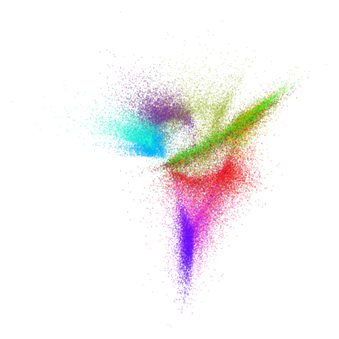
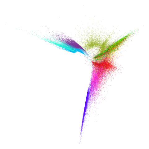
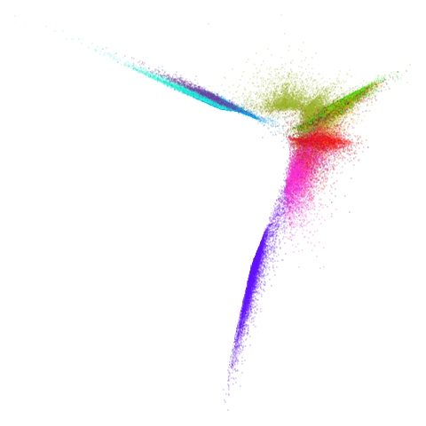
Sort of the same deal here as with mnist.
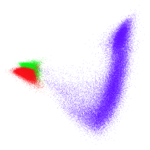
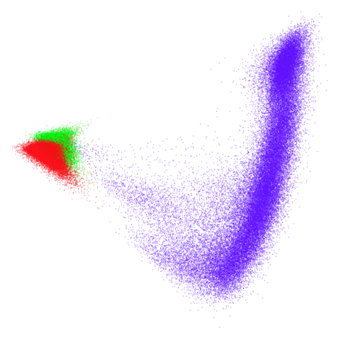
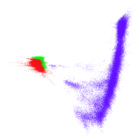
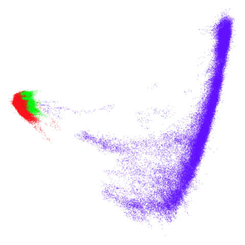
Another dataset I want to check is tomoradar. With the
Python UMAP package and this data, I have found this dataset will take
several minutes to converge. In uwot it can take over a
minute (the difference is due to the implementation of the spectral
decomposition). So like mammoth, this would be a good test
of whether convergence can be sped up. For this dataset, we use
n_neighbors = 50, because otherwise there is a disconnected
component. I want to compare the results here with a successful spectral
initialization because of the slow convergence.
tomoradar
| pca | 0 | 0.25 |
|---|---|---|
 |
 |
 |
| 0.5 | 0.75 | 0.9 |
|---|---|---|
 |
 |
 |
| 0.99 | 0.999 | 1 |
|---|---|---|
 |
 |
 |
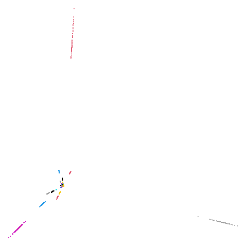
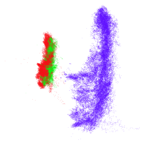
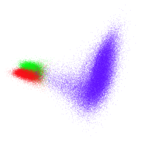
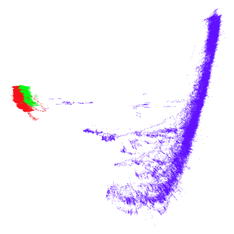
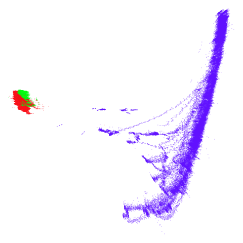
Even with a high graph_weight, the results resemble the
PCA results more than the spectral results. It seems like a situation
like with mammoth.
The next set of results are for datasets where you can’t do a
spectral initialization. uwot detects disconnected
components in the graph, steps in and makes you do PCA instead. So I
won’t try to go to graph_weight = 1. Also, nothing
interesting happens at graph_weight = 0.25 or
graph_weight = 0.75, so we can discard an entire row of
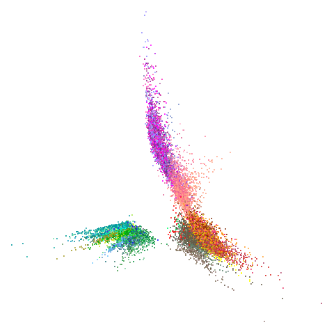
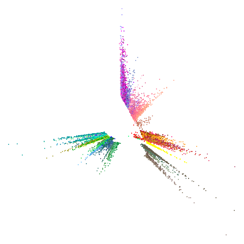
output. Without any ground truth to compare to, I am just looking for a
suitably “spectral-like” result at high graph_weight:
pointy, spiky, radial, etc. especially compared to the more diffuse PCA
results.
tasic2018
| pca | 0 | 0.5 |
|---|---|---|
 |
 |
 |
| 0.9 | 0.99 | 0.999 |
|---|---|---|
 |
 |
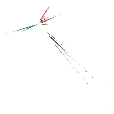 |
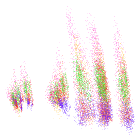
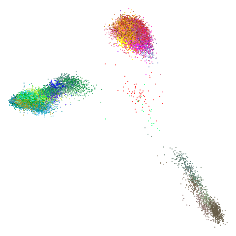
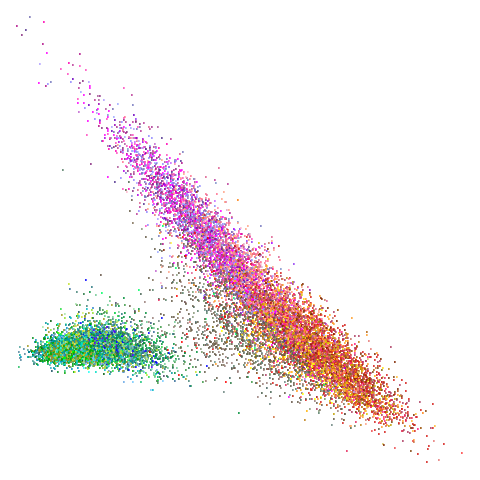
Ok, similar pattern emerges. We do have a successful enough looking
spectral shape at higher graph_weight values (and these all
converged quickly). Lower values inject some more PCA-like structure
into things.
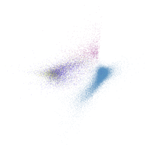
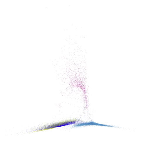
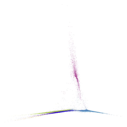
macosko2015 and its PCA-reduced version are all fully
connected, but I am including them here because they are transcriptomics
datasets like tasic2018.
macosko2015pca100
| pca | 0 | 0.5 |
|---|---|---|
 |
 |
 |
| 0.9 | 0.99 | 0.999 |
|---|---|---|
 |
 |
 |
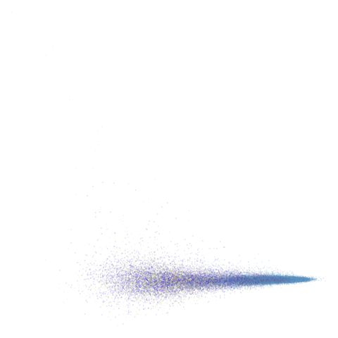
macosko2015 looking reliably terrible even in spectral
form, but macosko2015pca100 seems in line with the other
datasets.
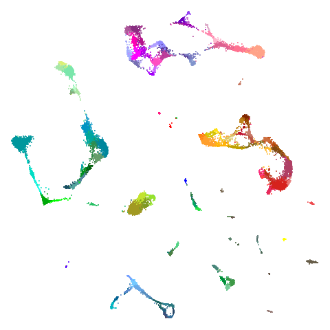
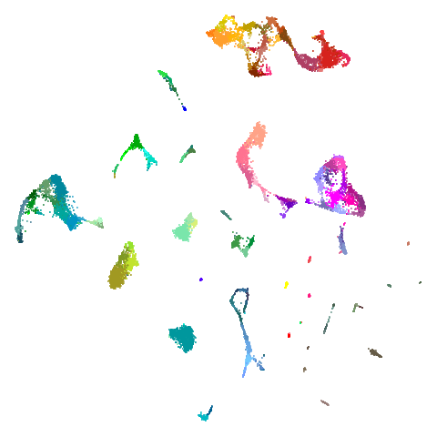
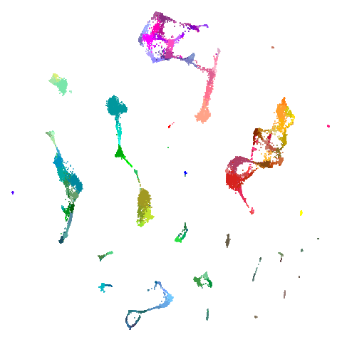
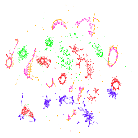
Overall, the initialization is doing what I want it to do with “real” datasets at least. Does it translate into different results when fed into UMAP?
UMAP
These are the UMAP embeddings of the datasets with the
initializations above. I use umap2 with the same nearest
neighbors that produced the initialization (but no mid-near neighbors).
The only deviation from default values is to use
rng_type = "deterministic" to remove any effect of random
numbers (which can’t always be controlled with multiple threads even
with the same seed). This probably introduces some other bias, but is
probably ok.
There is also one change for norb only. It never does
well with n_neighbors = 15 so for that dataset, I set
n_neighbors = 50, to make the results more legible
(probably there are other datasets where I should do this).
In most cases, there is nothing too surprising about the results if you know how the initializations look.
mnist
| pca | 0 | 0.25 |
|---|---|---|
 |
 |
 |
| 0.5 | 0.75 | 0.9 |
|---|---|---|
 |
 |
 |
| 0.99 | 0.999 | 1 |
|---|---|---|
 |
 |
 |
In this case the PCA result has some unfortunate overlapping and breaking up of the clusters, so everything is an improvement on that.
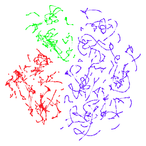
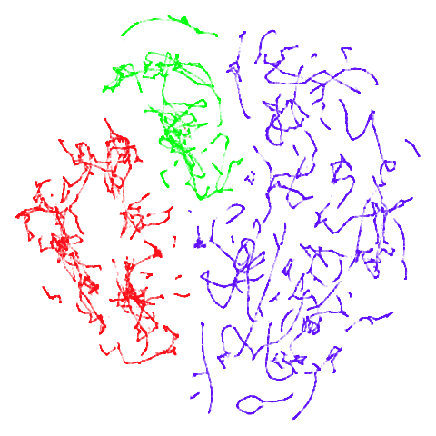
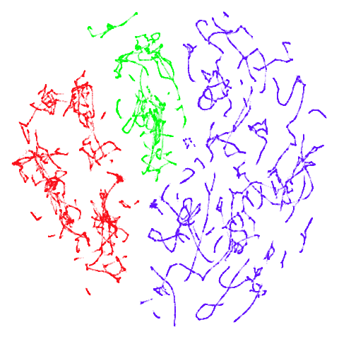
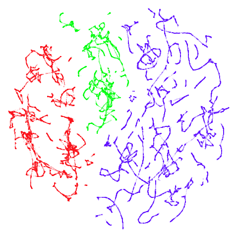
tomoradar
| pca | 0 | 0.25 |
|---|---|---|
 |
 |
 |
| 0.5 | 0.75 | 0.9 |
|---|---|---|
 |
 |
 |
| 0.99 | 0.999 | 1 |
|---|---|---|
 |
 |
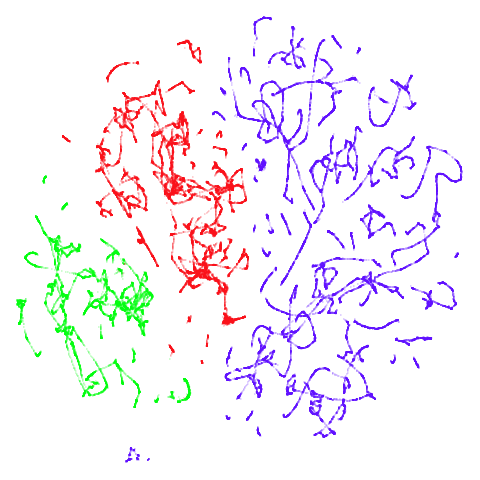 |
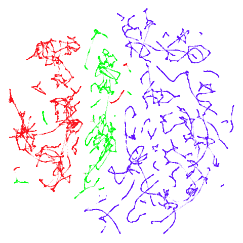
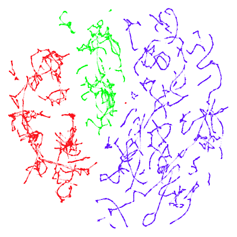
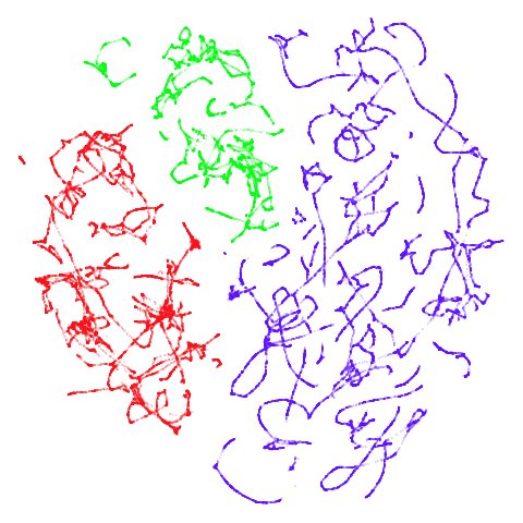
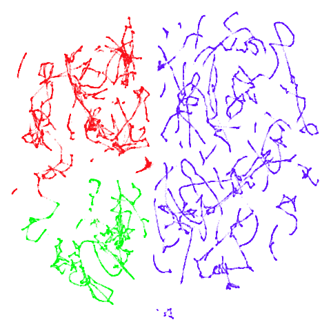
With the usual caveat that UMAP results for this dataset don’t look
like much of anything, at least with a
graph_weight = 0.999, you can get a result which resembles
what you get from spectral initialization. But it still takes around
20-30 seconds on my machine. That’s still somewhere around 2-3 times
faster than the pure spectral initialization, so a bit of a win.
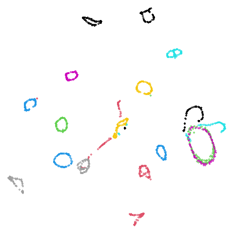
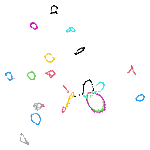
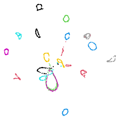
coil20
| pca | 0 | 0.5 |
|---|---|---|
 |
 |
 |
| 0.9 | 0.99 | 0.999 |
|---|---|---|
 |
 |
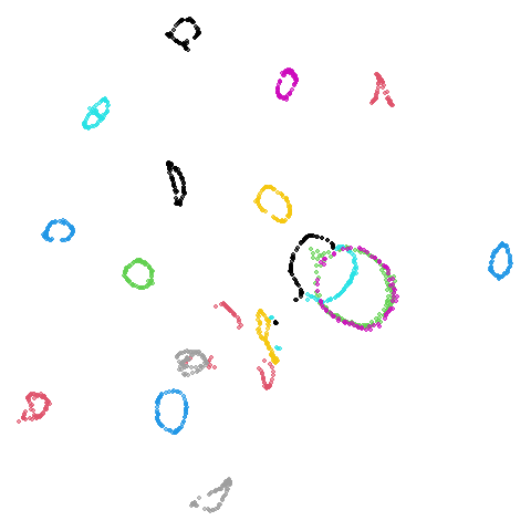 |
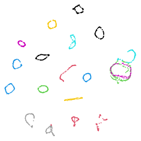
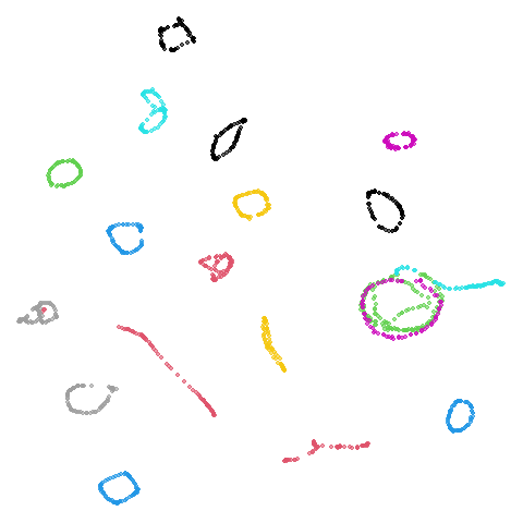
The downside of having disconnected components is that the clusters
are pretty free to move about relative to each other, so there’s not
always an obvious transition as graph_weight incraeses as
can be seen here.
norb
| pca | 0 | 0.5 |
|---|---|---|
 |
 |
 |
| 0.9 | 0.99 | 0.999 |
|---|---|---|
 |
 |
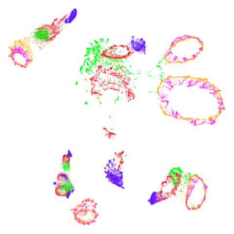 |
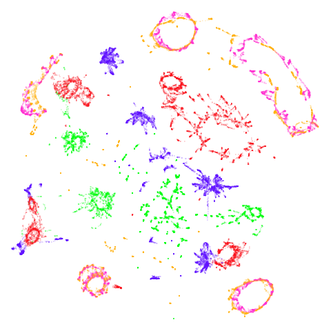
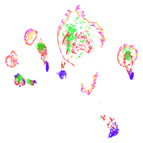
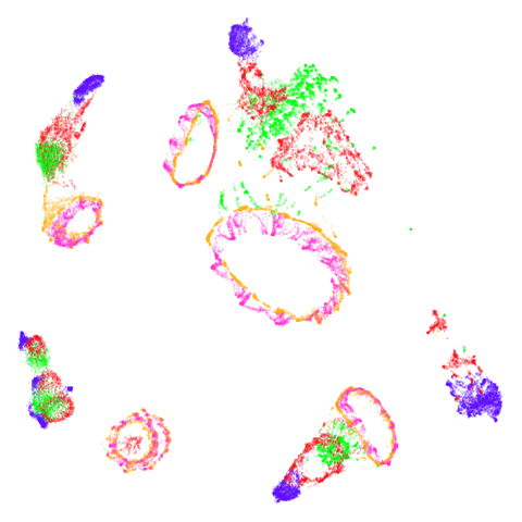
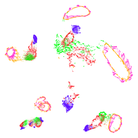
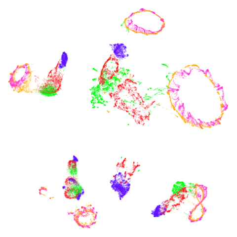
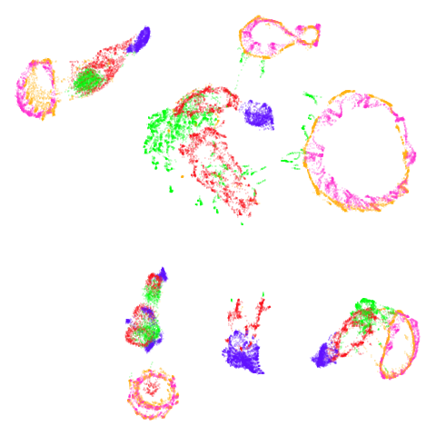
At least in the norb case, I think the mid-spectral
initialization improves on the PCA results, as it doesn’t break up the
pink/orange cluster in the top center.
tasic2018
| pca | 0 | 0.5 |
|---|---|---|
 |
 |
 |
| 0.9 | 0.99 | 0.999 |
|---|---|---|
 |
 |
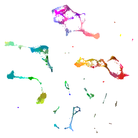 |
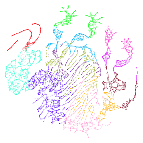
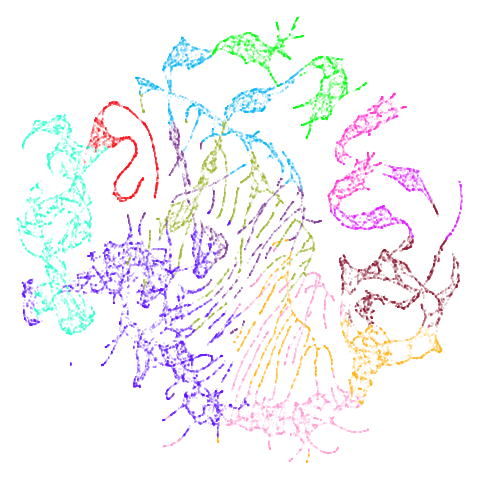
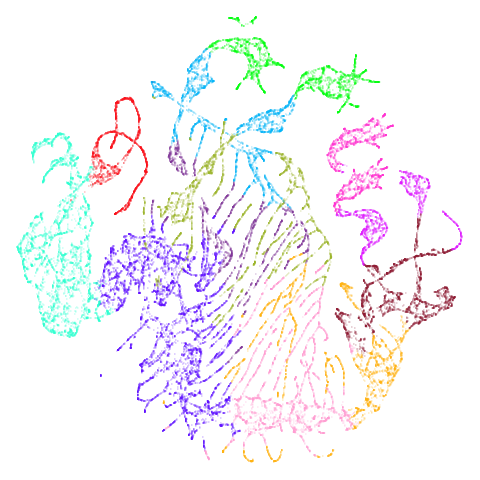
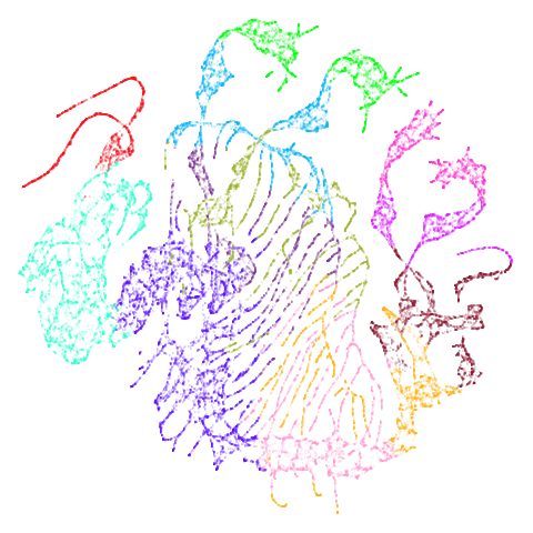
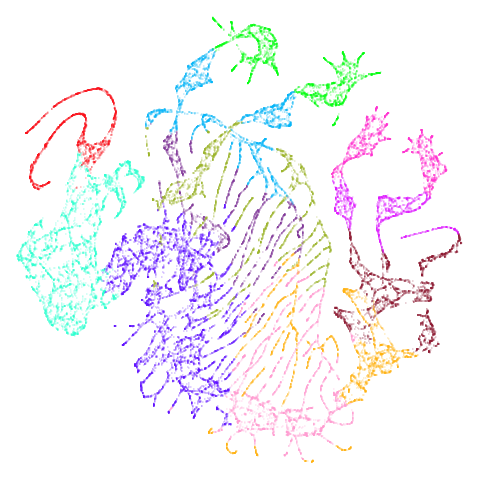
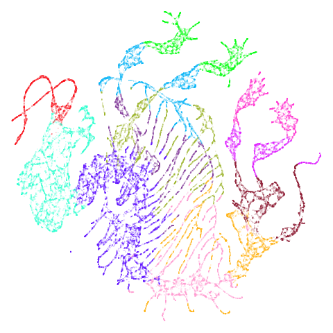
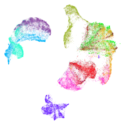
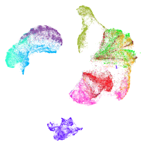
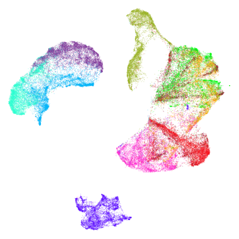
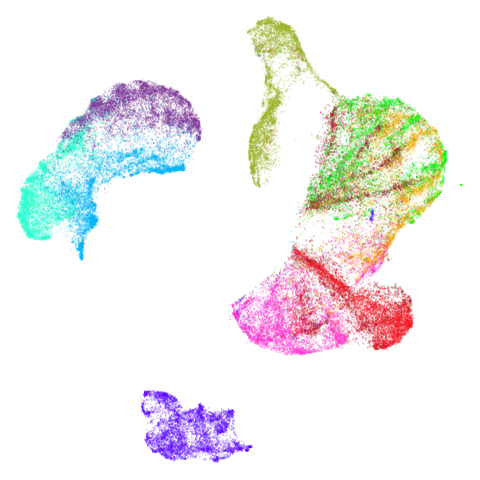
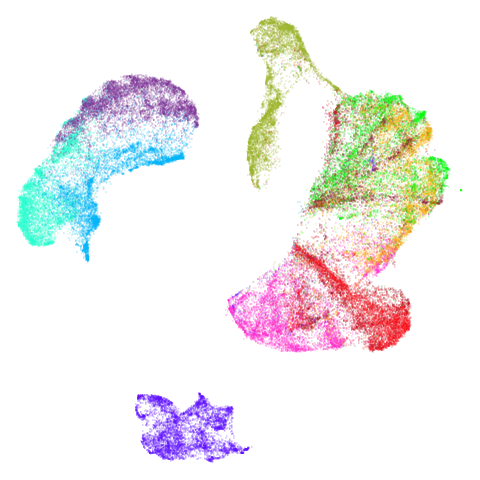
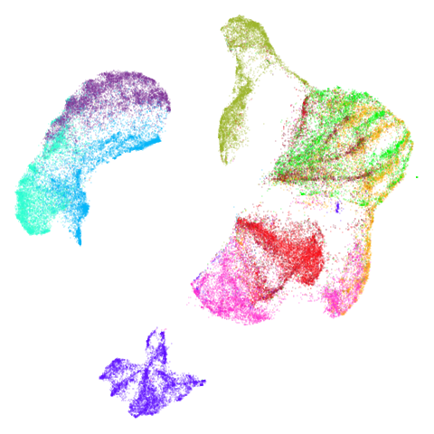
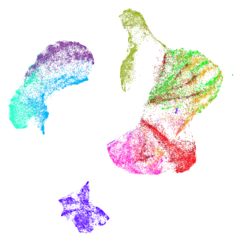
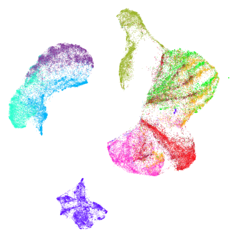
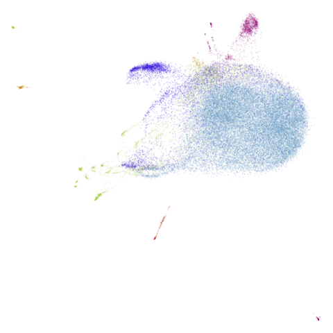
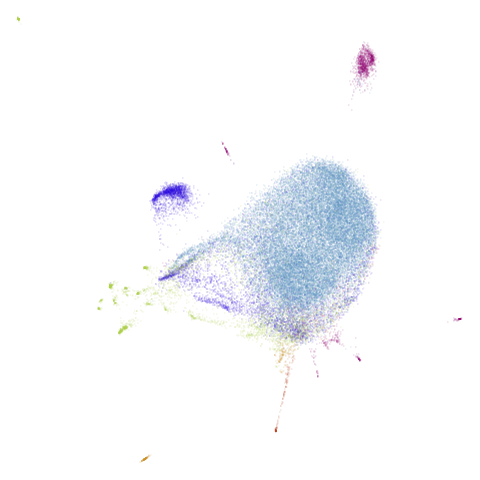
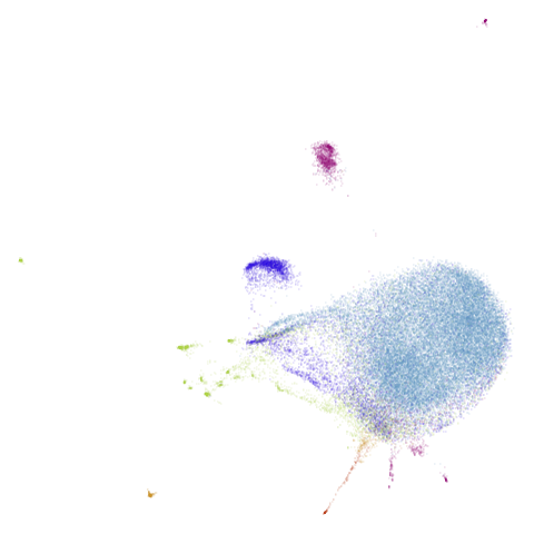
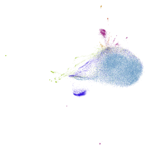
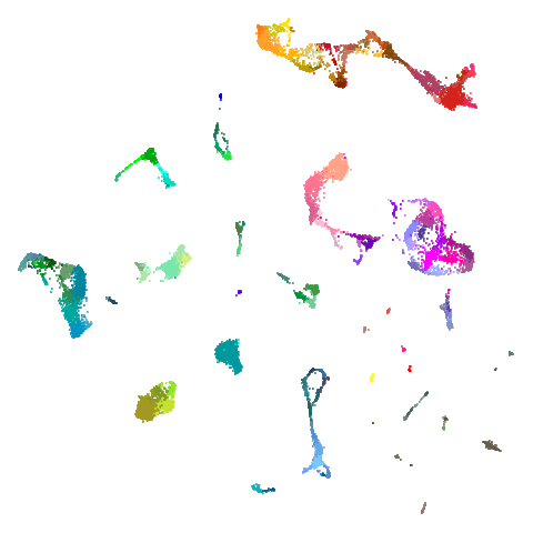
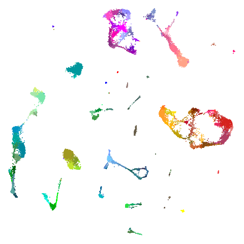
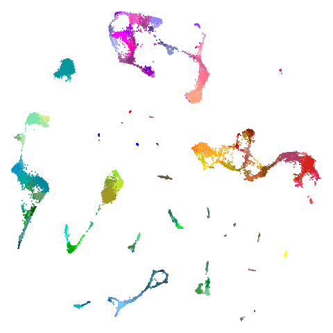
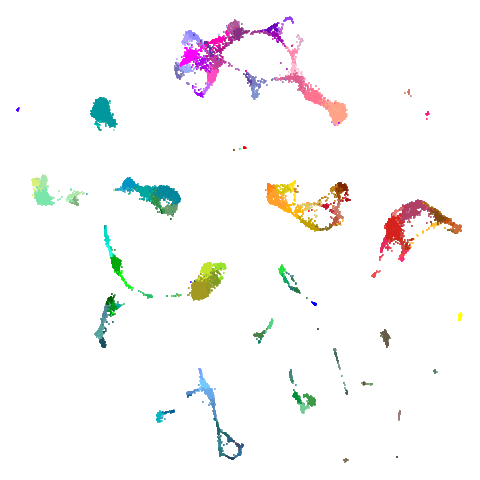
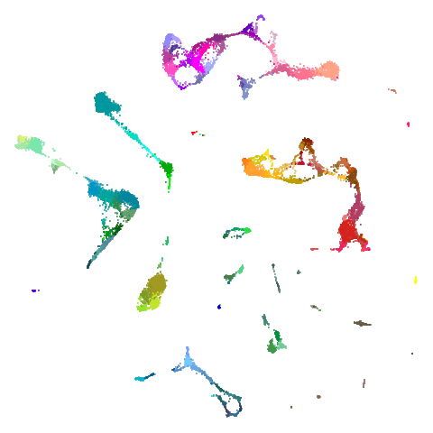
Cluster arrangement seems to be more consistently different in the mid-spectral initialization versus PCA in terms of the relative location of the orange-red versus the pink-purple cluster.
My conclusions from this set of results is that in most cases, there isn’t much difference between PCA and spectral initialization, but for some datasets, you can get some slightly different results with a spectral initialization and it might be improved over PCA, so having this available could be useful.
But not useful enough for me to add this to uwot
natively.
BMNN Initialization
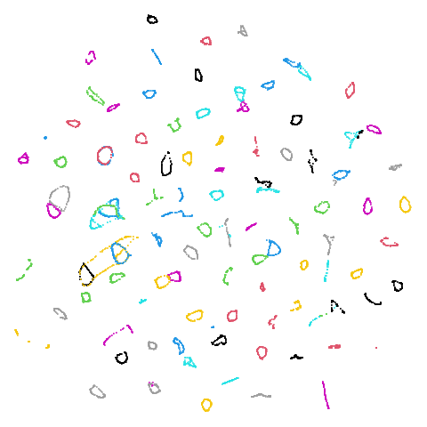
In the mutual nearest neighbors article, I lamented that focusing on MNN leads to more disconnections so initialization becomes even trickier. Could mid spectral initialization help?
Below I will consider 4 datasets which have a large number of disconnected components when using mutual nearest neighbors (and are disconnected even with just a knn graph).
For tasic2018 and norb I will use 50
nearest neighbors: norb because we know it does better that
way and tasic2018, just in case it will also show a
difference. For coil20 and coil100 I will use
15 nearest neighbors as these datasets do better with a smaller number
of neighbors. I will use 5 neighbors to ensure all items have at least 5
neighbors in the graph used for UMAP. See the MNN article for more
details on the procedure.
For each dataset we’ll consider all four combinations of the following settings:
- For the nearest neighbor graph, using either the k-nearest neighbors
or the balanced mutual nearest neighbor graph. In the results, the rows
will be marked as
knn<k>orbmnn-<k>-<m>respectively, wherekis either 50 or 15 andmis 5. - For the initialization, using either PCA or mid-spectral
initialization. For the mid-spectral initialization, the nearest
neighbor graph is either the knn graph or the balanced MNN graph.
graph_weight = 0.999in all these cases. In the results table, the columns are marked aspcaor0.999.
The question I want to answer here is: is initializing the coordinates using the neighbor graph better or at least different from using PCA?
Conclusions
If you have reason to want to avoid PCA initialization, but you have disconnected components in your nearest neighbor graph or the spectral initialization is having issues and failing to converge in a timely fashion, then using the mid-spectral initialization might be worth a try.
Unfortunately, like my agspectral attempt before, for
synthetic and manifold-like datasets, it may not be the right choice so
it’s not a guaranteed upgrade over spectral initialization in all
cases.
