UMAP with Mutual Nearest Neighbors

Introduction

Traditionally, dimensionality reduction methods make use of the k-nearest neighbors graph but there are some exceptions: Trimap and PaCMAP use an extended version of k-nearest neighbors, based on the “generalized” distances used in self-tuning spectral clustering, and PaCMAP goes further to also sample the kth closest neighbors from a locally sampled batch. LocalMAP also adjusts the neighbor graph dynamically during the embedding by sampling distances of the embedded points.

For the purposes of producing better-separated clusters, Dalmia and Sia (see also the article in the UMAP docs) consider the mutual nearest neighbors (augmented with some extra neighbors).

The way PaCMAP uses its neighbors is beyond the architecture of uwot to handle easilt, but the mutual nearest neighbors graph is something that uwot can deal with. As detailed in the article on uwot’s nearest neighbors format, we can provide as input a sparse distance matrix to represent nearest neighbors, giving substantial flexibility. However, it’s not always easy to take advantage of that. Here I will show some code that can generate a suitably-massaged mutual nearest neighbors graph and see if it has any effect on UMAP.

The Problem With Symmetrized k-Nearest Neighbors

Although in a kNN graph each item only has k neighbors, any workable dimensionality reduction working on the kNN graph as input will symmetrize that graph, otherwise optimization is difficult. The outcome of symmetrizing the knn graph is that if $j$ is a neighbor of $i$ in the kNN graph, $i$ is also guaranteed to be a neighbor of $j$ in the symmetrized graph and vice versa. If one item tends to show up in a lot of the kNN lists of multiple items, the symmetrization means that there can be up to $N$ edges involving that very popular item. These are called hubs and not only do they make search on the graph more difficult (that item will be likely to show up in most queries) but because for a given $k$ there are a limited number of edges to distribute over the dataset, some items are not getting their fair share. This is more likely to lead to outliers points that get embedded far away from the main body of the data as they have no particularly strong bonds to the rest of the data.

Mutual k-Nearest Neighbors

You can think of the mutual k-nearest neighbors graph (the MNN graph) as being a symmetrized kNN graph where edges only appear if item $i$ was a neighbor of $j$ and $j$ was a neighbor of $i$ : in the symmetrized kNN graph described above the requirement is only that $i$ be a neighbor of $j$ or $j$ be a neighbor of $i$ . This means that an item can have no more than $k$ mutual neighbors. Hub problem solved.

The Problem with Mutual k-Nearest Neighbors

The downside of the MNN graph is that even in very well-behaved kNN graphs, the MNN will contain several items with no edges to any other item: while they have $k$ nearest neighbors, none of those neighbors reciprocate. UMAP requires local connectivity, so it cannot handle a use case where we have such Billy no-mates items.

As a result, the Dalmia and Sia paper has to go to some extra lengths to augment the MNN graph with some extra nodes which you can see at their repo. This involves minimum spanning trees and Djikstra’s algorithm to add new nodes (and distances via the path length).

One alternative they consider is to take any fully disconnected nodes and re-add the first nearest neighbor. They cite a paper by de Souza, Rezende and Batista for this, but there’s no extra detail in that paper, the authors just note that they do this to avoid the disconnected nodes.

It should be said that this “adjacent neighbor” approach to MNN augmentation does not work very well, leading to a lot of disconnect components and small clusters of points scattered over the embedding. This is not very surprising.

Adding Back Extra Neighbors: The Balanced Mutual Nearest Neighbors Graph

As I don’t currently fancy implementing any of the path neighbor approach, I propose the following strategy: just add back more than one neighbor to disconnected nodes. In fact, we would probably do well to ensure every item in the dataset has at least $m$ neighbors where $m \lt k$ , not just items which are completely disconnected, as we can already see that items with only one neighbor don’t do a good job. Obviously adding back all the neighbors would recreate the original symmetrized kNN graph, so we want to keep $m$ small, but bigger than one.

To name this concept I am going with the “Balanced MNN graph” where “balanced” is meant to suggest that we are trying to ensure that no node is left too isolated in the MNN graph. To be specific with numbers I will refer to a ( $k$ , $m$ )-BMNN graph. I would welcome hearing if there is existing literature with a different (probably better) name.

Creating the BMNN

The basic formula for creating the BMNN graph is as follows:

Create the kNN graph.
Form the equivalent MNN graph.
Are there any nodes with fewer than $m$ neighbors? If not, we stop. Otherwise:
Add back the $m$ th-nearest neighbor from the kNN graph to each of those nodes.
Go to step 3.

The loop in steps 3-5 must terminate in $m$ steps: at worst, for items with 0 neighbors, we add all the $m$ -th nearest neighbors. For items with 1-( $m$ -1) neighbors, we don’t know if the $m$ -th nearest neighbor is already a neighbor. If it isn’t we are one step closer to termination. If it is, then adding the edge will do nothing. So we can’t add more than $m$ edges to any node and none of these nodes will get too many edges added.

Creating the MNN from the sparse kNN representation is easy, assuming your distances are symmetrical:

sp_mutual <- function(sp) {
  sp_t <- Matrix::t(sp)
  res <- sqrt(sp * sp_t)
  res
}

Balancing the MNN is a bit more involved, especially if you want it to be efficient and not do anything disastrous like accidentally attempt to turn your sparse matrix dense. We must go from 5 lines of code to more than 100. Below is the code for your delight and delectation. I may officially export this from uwot some day, but this remains an experiment for now for you to copy and paste.

Input to balance_mnn is:

nn_graph – the dense representation of the k-nearest neighbors, i.e. a list of two dense matrices, idx and dist both of dimensions (n, k). See the article on the nearest neighbor format for more. uwot exports in this format, and so does rnndescent.
k – optionally specify the size of the l nearest neighbors to use. If you omit this, all the neighbors in nn_graph will be used. Because generating nearest neighbors is time-consuming, you may wish to create a large neighbor graph once (e.g. set k = 50 or k = 150) and then use a smaller subset as the need arises (e.g. 15 is typical for UMAP). The nng helper function above can do this. Pro-tip: I use rnndescent::brute_force_knn to generate exact nearest neighbors for k = 150 and then save them once and for all. My now rather decrepit 8th gen Intel laptop still has enough juice to crank through datasets of up to 100,000 items and up to 10,000 features with 6 threads in a “reasonable” amount of time, where “reasonable” for me means anything up to a few hours, but not “going on holiday for two weeks”.
m – minimum number of neighbors to ensure each item has. This needs to be at least two.

One slightly weird thing about specifying m is that you will actually get back one less edge than the value you ask for. This is because in the dense format every item’s nearest neighbor is itself with a distance of zero. This disappears when we convert to the sparse format. As a result your dense k-nearest neighbor graph only contains $k-1$ different neighbors for each item. The self-neighbor thing counting as one of the neighbors is always how UMAP has done it, so we won’t be changing the habit of a lifetime. You will just have to remember to reproduce the “adjacent neighbor” method you must specify m = 2. The function won’t let you go lower than m = 2 anyway.

# create an m-balanced k-mutual nearest neighbors graph from the dense k-nearest
# neighbors graph `nn-graph`. m must be less than or equal to k. If `k` is not
# specified then all of the neighbors are used.
balance_mnn <- function(nn_graph, m, k = NULL) {
  if (m < 2) {
    stop("m must be at least 2")
  }

  if (!is.null(k)) {
    nn_graph <- nng(nn_graph, k)
  }
  k <- ncol(nn_graph$idx)
  if (m > k) {
    stop("m must be less than or equal to k")
  }

  # create the mutual neighbors as a sparse matrix
  # each item's neighbors distances are stored by column
  bmnn <- k_to_m(nn_graph)
  bmnn_adj <- sp_to_adj(bmnn)
  bmnn_edges <- colSums(bmnn_adj)
  too_few_edges_mask <- bmnn_edges < (m - 1)

  # add edges back from the knn graph to "fill up" any items with too few edges
  # do it one column at a time to avoid over-filling any one item
  for (l in seq(from = 2, to = m)) {
    if (sum(too_few_edges_mask) == 0) {
      break
    } else {
      message("Iter ", l, " cols to process: ", sum(too_few_edges_mask))
    }

    knn_idxl <- nn_graph$idx[, l]
    masked_knn_distl <- nn_graph$dist[, l] * too_few_edges_mask
    masked_knn <- vec_to_sp(knn_idxl, masked_knn_distl)
    knn_adj <- sp_to_adj(masked_knn)

    mk_adj <- bmnn_adj + knn_adj
    bmnn <- bmnn + masked_knn
    bmnn@x <- bmnn@x / mk_adj@x

    bmnn_adj <- sp_to_adj(bmnn)
    bmnn_edges <- colSums(bmnn_adj)
    too_few_edges_mask <- bmnn_edges < (m - 1)
  }

  bmnn
}

## Helper functions

# truncate a dense neighbor graph to the first k neighbors
nng <- function(graph, k) {
    list(idx = graph$idx[, 1:k], dist = graph$dist[, 1:k])
}

# convert a dense knn graph to a sparse matrix format
# NB neighbors are stored by column
nng_to_sp <- function(graph, nbrs = NULL) {
  if (!is.null(nbrs)) {
    graph <- nng(graph, nbrs)
  }

  idx <- graph$idx
  dist <- graph$dist
  n_nbrs <- ncol(idx)
  n_row <- nrow(idx)
  n_ref <- nrow(idx)
  i <- as.vector(idx)
  j <- rep(1:n_row, times = n_nbrs)

  x <- as.vector(dist)
  keep_indices <- !is.na(x)
  i <- i[keep_indices]
  j <- j[keep_indices]
  x <- x[keep_indices]
  res <- Matrix::sparseMatrix(i = i, j = j, x = x, dims = c(n_row, 
      n_ref), repr = repr)
  Matrix::drop0(res)
}

# convert a sparse knn matrix to the mutual nearest neighbors graph
sp_mutual <- function(sp) {
  sp_t <- Matrix::t(sp)
  res <- sqrt(sp * sp_t)
  res
}

# convert a dense kNN graph to a mutual nearest neighbors graph
k_to_m <- function(graph, nbrs = NULL) {
  sp <- nng_to_sp(graph, nbrs)
  res <- sp_mutual(sp)
  res
}

# convert sparse matrix to an adjacency matrix (1 if there's an edge, 0 otherwise)
sp_to_adj <- function(sp) {
  spi <- sp
  spi@x <- rep(1, length(spi@x))
  spi
}

# convert the vector of values x to a sparse matrix with where the row is given
# by the equivalent value in the vector i, and the column is the index of the
# value in the vector x. The resulting matrix is a square matrix with the same 
# number of rows as the length of x.
vec_to_sp <- function(i, x) {
  n_row <- length(i)
  j <- 1:n_row

  keep_indices <- !is.na(x)
  i <- i[keep_indices]
  j <- j[keep_indices]
  x <- x[keep_indices]
  res <- Matrix::sparseMatrix(
    i = i,
    j = j,
    x = x,
    dims = c(n_row, n_row),
    repr = "C"
  )
  Matrix::drop0(res)
}

Disconnections and the Question of Initialization

Dalmia and Sia note that using a MNN graph leads to many disconnected components, which can cause issues with the default spectral initialization in UMAP. Their approach creates a connected graph to get round this problem. An alternative I pursue in all the results here is to always initialize from the first two components of PCA. Even in the case of the kNN graph, you can still get disconnected components for a given value of n_neighbors, and uwot will fall back to PCA in this case anyway.

Working with the BMNN

Putting this together, my recommended workflow is:

library(rnndescent)
librart(uwot)
# get the approximate knn: use as many threads as you want
data_knn_15 <- rnndescent::rnnd_knn(data, k = 15, n_threads = 6)
# or if you have time on your hands
# data_knn_15 <- rnndescent::brute_force_knn(data, k = 15, n_threads = 6)

pca_init <- umap2(data, nn_method = data_knn_15, init = "pca", n_epochs = 0)

# Normal UMAP
data_umap <- umap2(data, nn_method = data_knn_15, init = pca_init)

# Create the (15, 5)-balanced MNN
data_bmnn_15_5 <- balance_mnn(data_knn_15, k = 15, m = 5)

# UMAP with BMNN
data_bmnn_umap <- umap2(data, nn_method = data_bmnn_15_5, init = pca_init)

In the work presented by Dalmia and Sia, multiple choices of k are tried (from 10-50) and some changes to min_dist. I will stick with k = 15 for all the results shown here.

MNIST Example

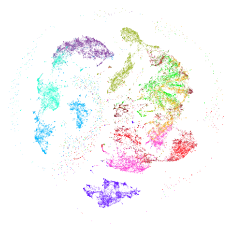
Does the BMNN graph produce results that differ from the kNN graph? Let’s compare the UMAP embeddings of the MNIST digits and Fashion MNIST datasets using the kNN graph and the BMNN graph. From left to right we have the original UMAP embedding, the embedding using the (15, 2)-BMNN graph which should give similar results to the MNN+adjacent neighbors approach used by Dalmia and Sia, and the an embedding using the (15, 5)-BMNN graph which (I hope) should give a more “connected” embedding. You can click on any of the images to see a (slightly) larger version.

Dataset	15-NN	(15,2)-BMNN	(15,5)-BMNN
MNIST
fashion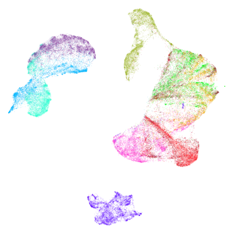

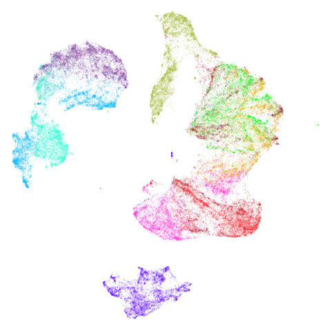Although it’s not that easy to see unless you click on the image, the (15,2)-BMNN results do show a sprinkling of outlier points throughout the embedding. This confirms the observations of Dalmia and Sia and so this doesn’t seem like a promising approach. I won’t bother showing results for (15,2)-BMNN graphs going forward. The (15,5)-BMNN on the other hand seems quite well behaved. Now, if you were to say “I put it to you that it doesn’t look very different from the normal UMAP results” I would have to agree with you. But there is perhaps slightly more separation of the clusters and some finer detail? Possibly that’s entirely within the expected variation of a given UMAP run.

Fortunately there are some datasets where we do see more a difference.

COIL-20 and COIL-100

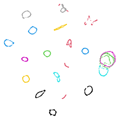
Embedding COIL-20. and COIL-100 show a series of loops, but some of which typically get a bit tangled up together or mangled. If ever there were some datasets that might benefit from focusing on the mutual neighbors, it’s these two.

Dataset	15-NN	(15,5)-BMNN
coil20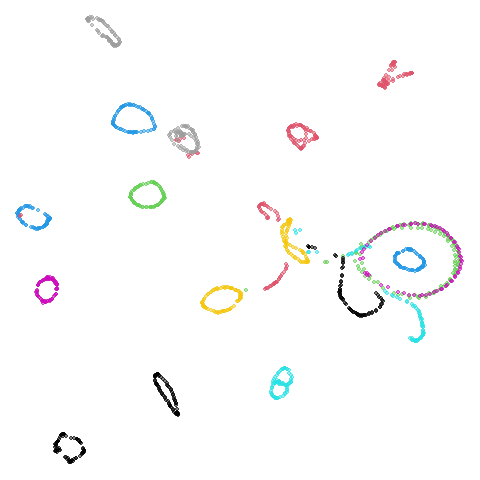
coil100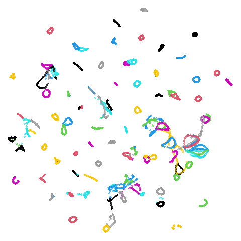

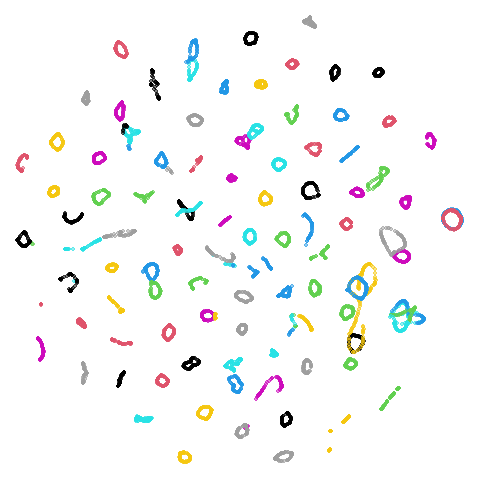I no longer feel like I am lying to myself when I say I can see a difference between the two embeddings. The BMNN graph definitely seems to have untangled the loops a bit more.

Disappointing Results

There are some datasets which UMAP struggles to produce useful results for. These include:

the image dataset CIFAR-10 where I just wouldn’t expect looking at Euclidean distance in the raw pixel space to produce anything of value (and it doesn’t).
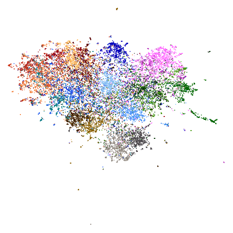
the text dataset 20Newsgroups that I have attempted to process with UMAP in the past: this version was cleaned, had TF-IDF applied and then L2 normalized. Clusters do appear but they aren’t very well-separated. This appears in the Dalmia and Sia paper with a different processing (and also in the PaCMAP paper with a different processing again) without looking terribly attractive.
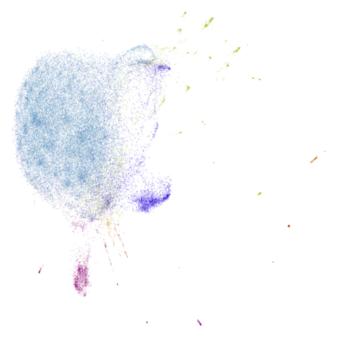
The scRNA-seq data macosko2015, which in its raw form has around 3000 columns. It shows extreme hubness: the MNN graph (with k = 15) results in 89% of the dataset being entirely disconnected! A corresponding problem is that you have to be quite careful with how large m is in the BMNN: as the vast majority of edges in the kNN graph are pointing towards the hubs, even a small number of additions of kNN edges back can lead to a hub in the BMNN. The symmetrized kNN graph has a hub with 10,000 edges associated with it (around 20% of the dataset). The BMNN graph with m = 5 reduces that, but the hub still has 4,000 edges.
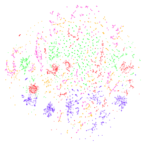
macosko2015 visualizes more nicely with some PCA as the hubness is greatly reduced (I am agnostic on if this representation more faithfully represents the biological reality). so I also include the same dataset after reducing to 100 dimensions with PCA.
The Small NORB image dataset of objects, is not as challenging as the other datasets listed here. In fact, it is slightly COIL-ish in that it already shows some loops and other structure in UMAP. So could using the MNN graph improve matters further as it has for COIL-20 and COIL-100?

Dataset	15-NN	(15,5)-BMNN
norb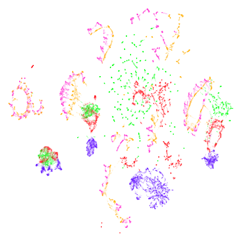
macosko2015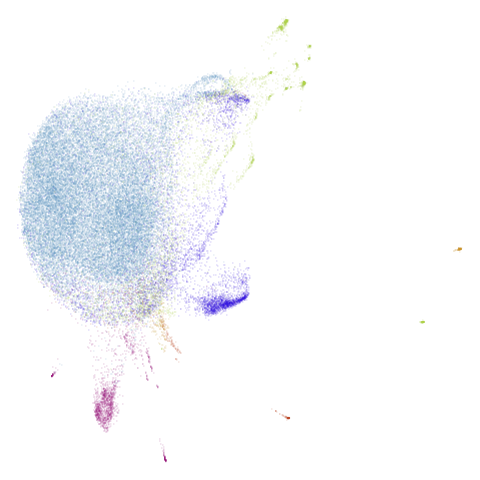
macosko2015pca100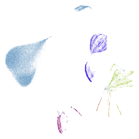
20NG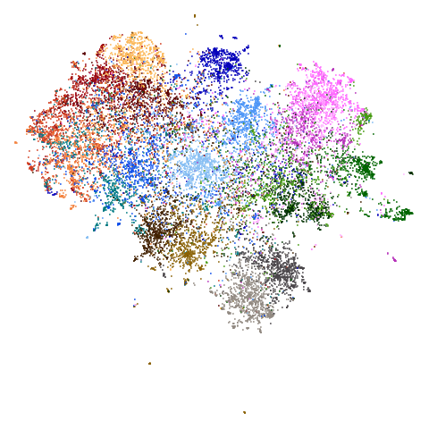
cifar10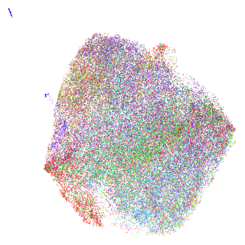

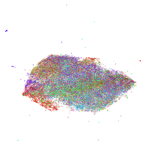Ok, so it turns out that the BMNN graph doesn’t really help in any of these cases. norb is particularly disappointing in that it noticeably makes things worse.

For macosko2015, pretty much nothing happens, except the big blue round cluster has got some slight mottling where it seems like some kind of fine(ish) structure is forming, which might translate to clusters. I couldn’t tell you if it was biologically relevant though. I tested whether the hubness that is present in the kNN and creeps back into the BMNN is a determinant of this embedding by creating a BMNN where edges were added back not in order of shortest distance, but in smallest k-occurrence, i.e. items that appear the least often in the kNN graph. This reduces the maximum edge count in the BMNN to around 200 (a nearly 20-fold drop), but the embedding looks very similar to the vanilla UMAP result:

macosko2015 (15, 5)-koBMNN

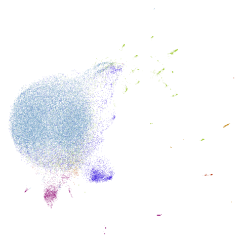I include this image only because this is evidence against my long-held belief that hubs in the kNN graph are a problem for UMAP, so this is a good visualization for me to stare at the next time I start going down this road. macosko2015pca100 shows very little change also.

For 20NG and cifar10 the only effect is to make the main blob of data more compressed in the middle of the plot, due to extra small clusters now being located at the edges. While not attractive, this could be indicating some anomalous clustering in these small subsets, which might be worth investigating further. For example, these could be duplicates or close duplicates. I haven’t actually done that investigation though so I can’t say if that’s the case.

norb revisited

December 29 2024: Looking further at the norb results, I couldn’t shake the feeling that the way the results were broken up when going to the BMNN result indicated that the n_neighbors was set too low. So let’s try with n_neighbors = 50. I will set the BMNN to (50,5). Possilbly, a larger values of k means we also need a larger value of m to get a good result but let’s see if we can get away with just changing one parameter.

Dataset	50-NN	(50,5)-BMNN
norb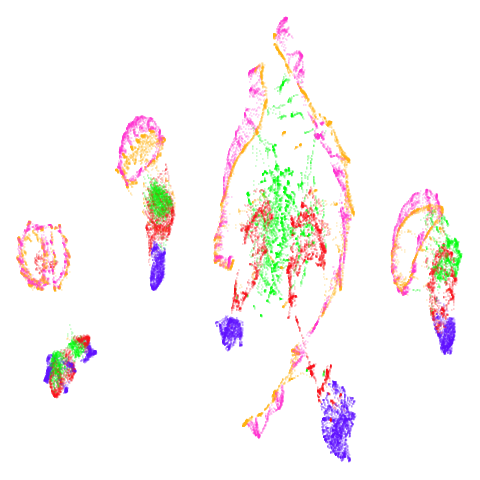

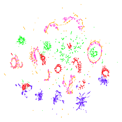Ok, I am back to not hating BMNN for norb. Results are a bit messy, but it’s definitely doing something: the BMNN separates out the objects based on their class (the colors) to a much greater extent than the kNN version, which has the results in more cleanly separated clusters but with the classes more intertwined.

Conclusions

Using the BMNN to approximate the MNN is a mixed bag. In some cases it can help, but in others it either does very little, or can make things worse – although there’s always a chance that this could be a diagnostic of unusual structure in the data.

Also worth noting is that the BMNN graph is much sparser than the symmetrized kNN graph that UMAP uses by default. In the examples here the (15, 5)-BMNN graph has around 1/3-1/2 the number of edges of the kNN graph. This can give a moderate speedup in the UMAP embedding step: around 25-50%.

BMNN results are certainly not as visibly different as that seen in the Dalmia and Sia paper. Why is this? It could be that I need to tweak k and m specifically for each dataset although that makes the BMNN approach very unappealing. It could also be that a spectral initialization using the BMNN approach would give different results, but in order to do that, we would need a strategy to form a fully connected graph Laplacian. In general that would be a useful thing to generate from any neighbor graph, but it seems like something that is more suited to a graph or nearest neighbor package (like rnndescent) than uwot itself.

Certainly the BMNN is no panacea to datasets that don’t show much structure, but that was a pretty forlorn hope. My advice would be that if your UMAP result does show some kind of structure, then it’s worth trying the BMNN as it’s not difficult or time-consuming to generate. As the norb example shows, if the BMNN destroys the clustering, that could be a sign to try again with a larger values of n_neighbors.

The Balanced Mutual Nearest Neighbors Graph

December 25 2024