December 27 2024: Updated to use umap2 and with
better images.
Introduction
The default initialization for UMAP uses the eigenvectors of a normalized graph Laplacian of the sparse affinity matrix. This normally works well except when:
- The graph has disconnected components, in which case you really have
multiple separate graphs. In
uwot, there is a risk that the RSpectra can have trouble converging under these circumstances. - Even with a connected graph, there can sometimes be convergence issues, which I have tried to mitigate. However, there is a still a risk of a very long initialization, and possibly a hang. Unfortunately, interrupting RSpectra can result in requiring the entire R session to be lost.
PCA Initialization
An alternative to using the spectral initialization is to use PCA,
although depending on the scaling of your input variables, this could
lead to a quite spread-out initial set of coordinates, which can be hard
to optimize. For the related technique t-SNE, Kobak and
Berens recommend scaling the PCA results so that the standard
deviation for each dimension is 1e-4. You can get that
behavior in uwot by using the umap function
with init = "spca" or umap2 with
init = "spca", init_sdev = 1e-4.
Changes with umap2
Based on some years of experience, the umap2 function
has some slightly different defaults which I recommend over
umap. For more on the umap2 function, see the
umap2
article. But I recommend using init = "pca". At some
point after I wrote uwot (or I just never noticed), the
Python UMAP package added an extra scaling of coordinates so that they
are contained in a bounding box of side length 10. This is now the
default with umap2 and seems to work pretty well.
All the results shown on this page now use umap2.
If you are still using umap
If you are still using umap, then the
init = "spca" option there works ok, but the standard
deviation of 1e-4 may be too small for some datasets. If
you see results where you are suspicious that clusters are being broken
up, I recommend trying with value of init_sdev of
1e-2, 1 or 2.5. If you want to
use the Python UMAP-style scaling with umap, you can get it
by setting init_sdev = "range", and is probably the best
choice.
The Approximate Global Spectral Initialization
PCA is a solid choice for initialization when spectral embedding fails. But using PCA ignores the information in the affinity matrix that might be useful for initialization: for example, when using supervised UMAP or mixing different types of distance metrics. And conceptually, using the affinity matrix has a lot of appeal. Dzwinel and co-workers describe a very fast multi-dimensional scaling-like method called ivhd which generates a connected graph, by only knowing only a few neighbor and non-neighbor points and pretending the target distances are 0 and 1, respectively. Similar theoretical support for this is given by Linderman and co-workers. On the basis of this work, I have implemented an “approximate global” spectral method of initialization: which is a very minor modification of the standard spectral initialization:
- All non-zero elements of the affinity matrix are set to 1.
- A random number of the zero elements are set to 0.1, at a rate of
n_neg_samplesfor each positive edge in the graph. This is consistent with the ratio of neighbor to non-neighbor edge sampling during optimization and, if using a default value ofn_neg_samples, is a similar order of magnitude as the ratio of neighbor to non-neighbor entries in the graph that is used with ivhd. - Theoretically, this should be enough to guarantee a graph with a single component. The spectral initialization is carried out.
- After initialization, the original affinity matrix is used for optimization.
You can get this behavior in uwot with
init = "agspectral".
Laplacian Eigenmap
Another option for a connected graph is to use a variation on the
normalization used in the graph Laplacian to get something close to Laplacian Eigenmap
with init = "laplacian". In Luxburg’s
spectral clustering tutorial (PDF) this form of normalization is
recommended over that used in the init = "spectral"
normalization. So we’ll try it here and see if it makes any
difference.
Random Initialization
If all else fails, you can use random initialization. In the spirit
of generosity, uwot offers two types of random
initialization. The first is that used by UMAP, which uses a random
uniform distribution between -10 and +10 along each axis. You can get
this with init = "rand". Alternatively, there is the method
favoured by LargeVis (and used by default with lvish),
which is to use a Gaussian distribution with standard deviation 1e-4.
This is also the method used by t-SNE. You can get this by setting
init = "lvrand".
To summarize your options:
# Default initialization: use spectral initialization if possible
# falling back to scaled PCA if multiple components are found in the graph
embedding <- umap2(data)

# same as the above
embedding <- umap2(data, init = "spectral")

# use (scaled) PCA: defaults are different between umap and umap2
embedding <- umap2(data, init = "pca")

# If you want to use `umap` then you can use the following:
# umap with default scaled PCA
embedding <- umap(data, init = "spca")
# equivalent to:
embedding <- umap(data, init = "pca", init_sdev = 1e-4)
# but this might be a better choice of settings
embedding <- umap(data, init = "pca", init_sdev = "range")

# use an "approximate global" spectral initialization that should be applicable
# even under conditions where "spectral" fails and has to use spca
embedding <- umap2(data, init = "agspectral")

# use a Laplacian Eigenmap style initialization, which will also fall back to
# spca if it has to
embedding <- umap2(data, init = "laplacian")

# use random initialization, UMAP style
embedding <- umap2(data, init = "rand")
# use random initialization, t-SNE/LargeVis style
embedding <- umap2(data, init = "lvrand")
Below, we’ll explore the effect of these settings. For more details on the datasets, see the examples page.
Apart from changing init, mainly default settings where
used. To save a bit of time, I used pre-calculated exact nearest
neighbors, but I don’t expect that to have a major effect on the
results. Some typical commands using the iris dataset would
be:
Datasets
For details see the examples article.
Spectral vs PCA
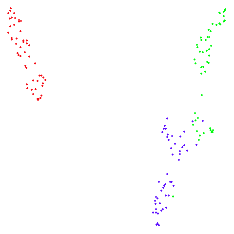
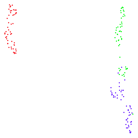
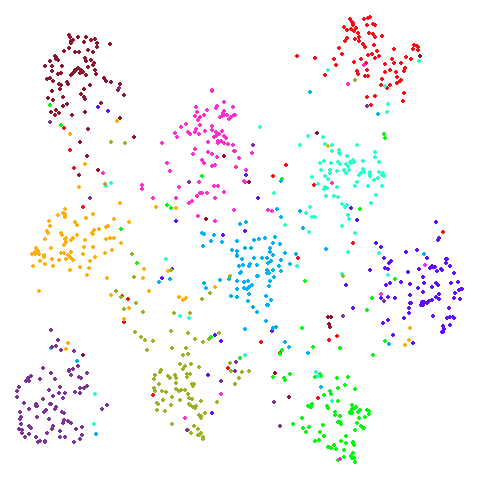
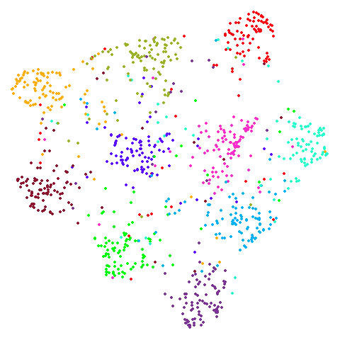
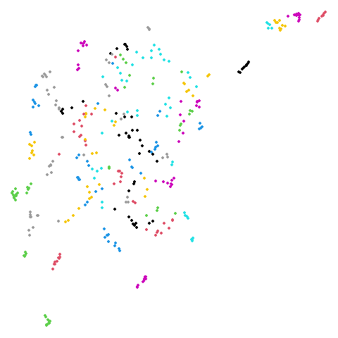
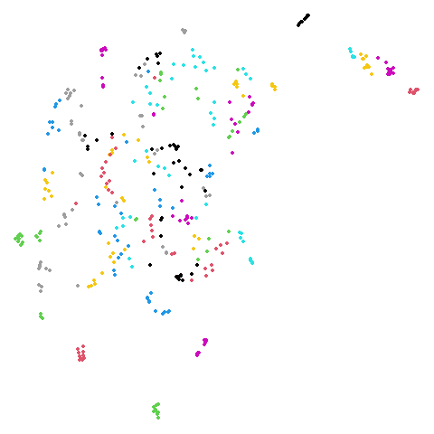
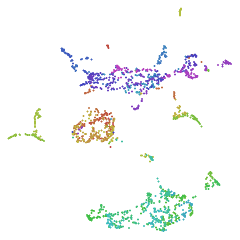
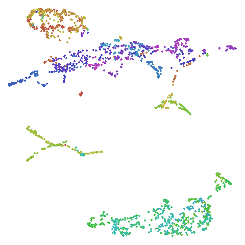
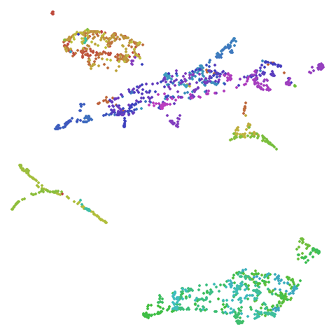
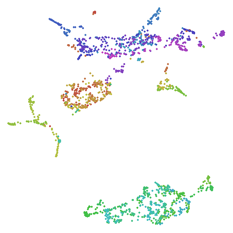
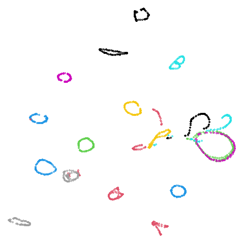
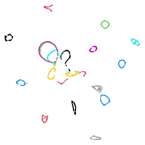
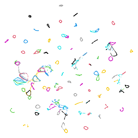
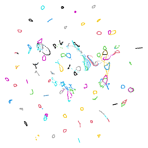
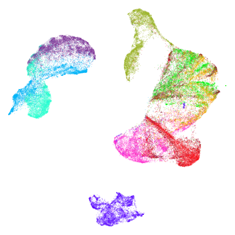
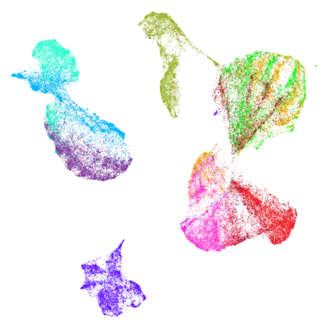
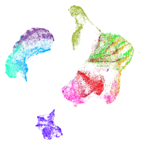
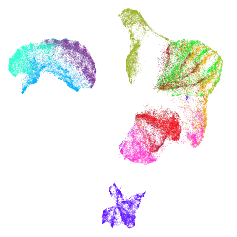
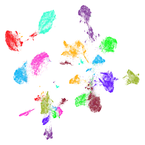
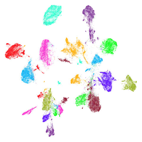
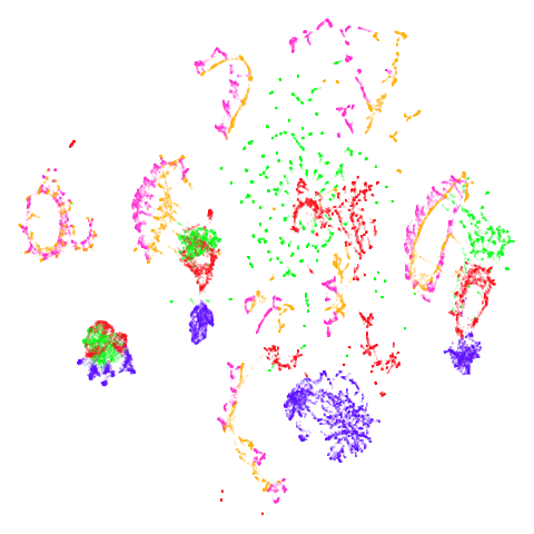
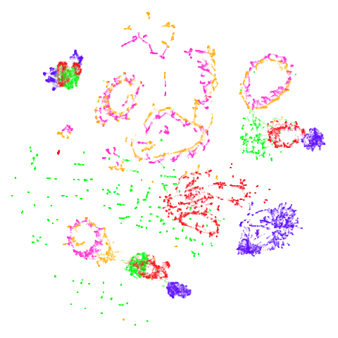
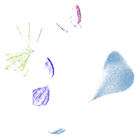
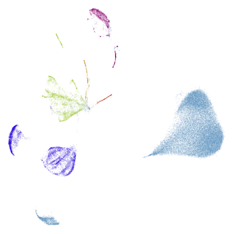
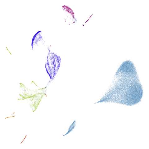
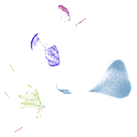
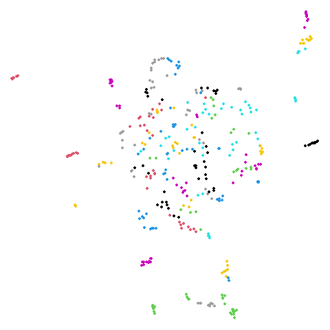
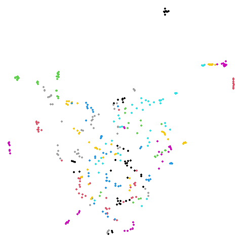
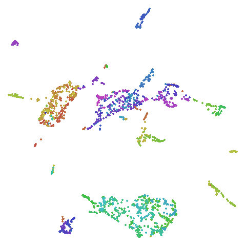
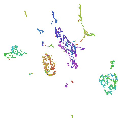
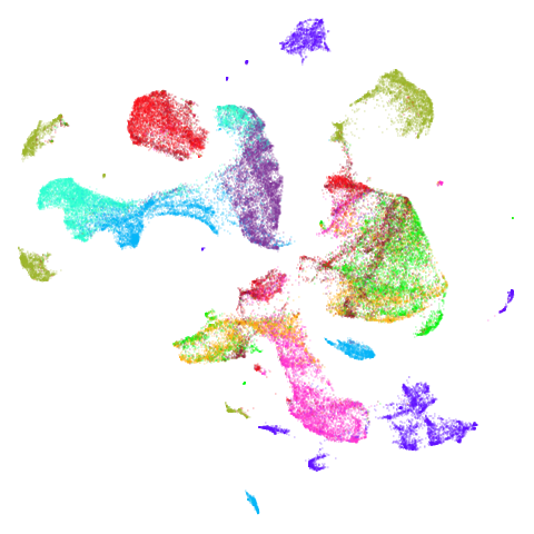
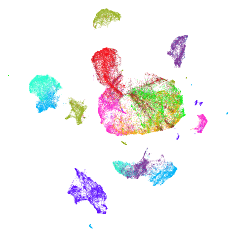
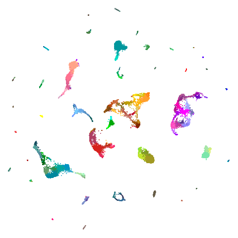
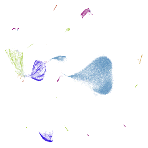
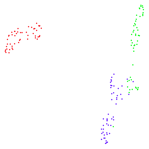
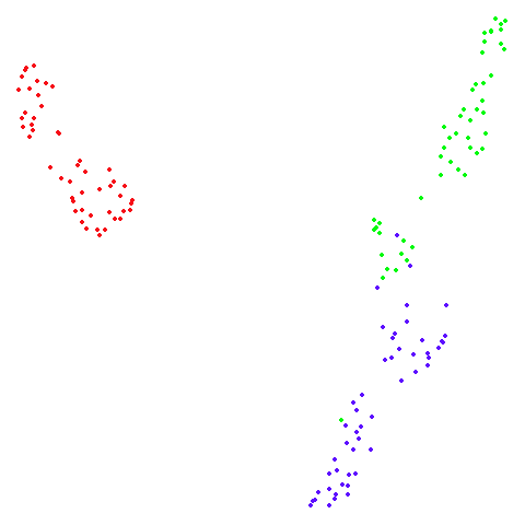
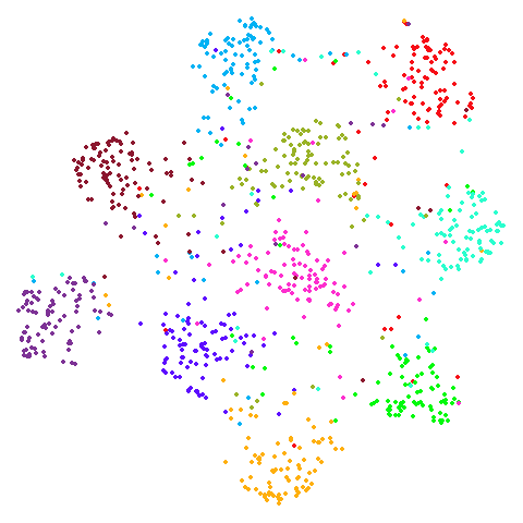
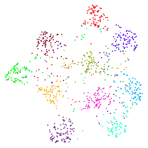
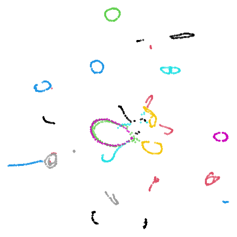
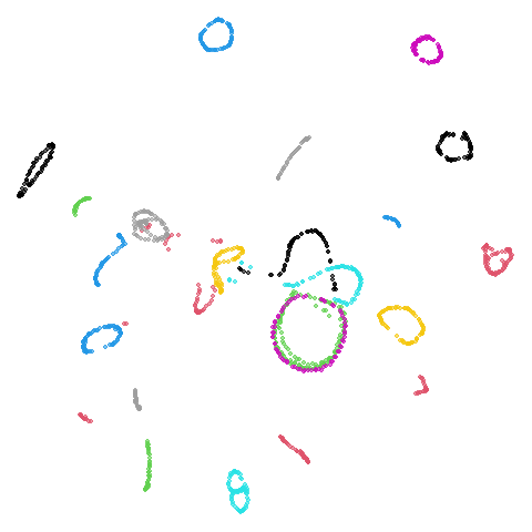
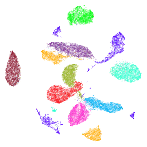
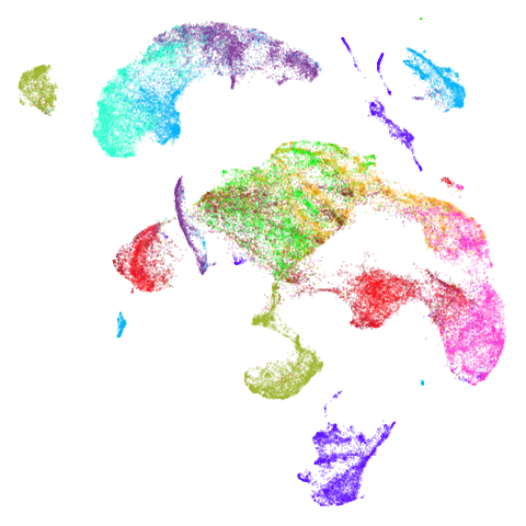
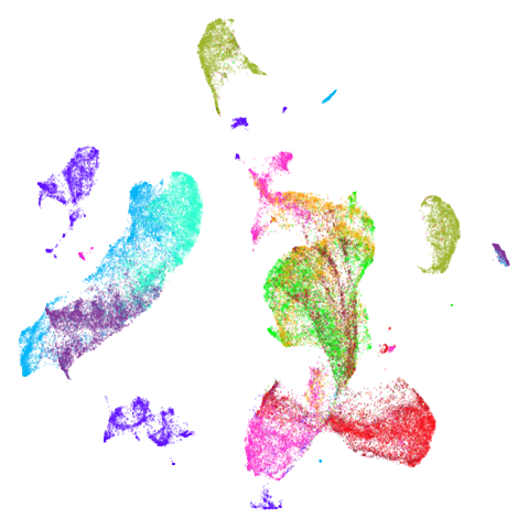
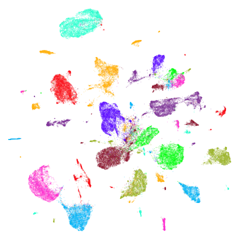
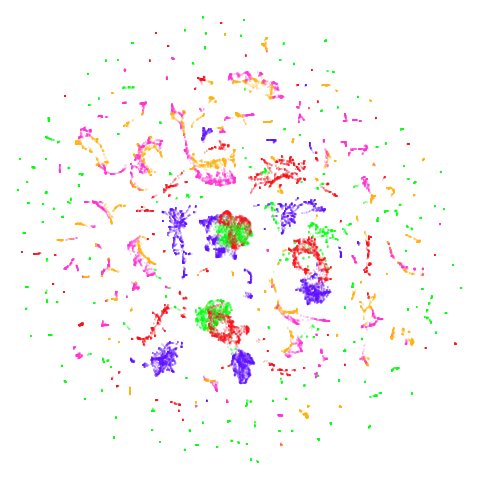
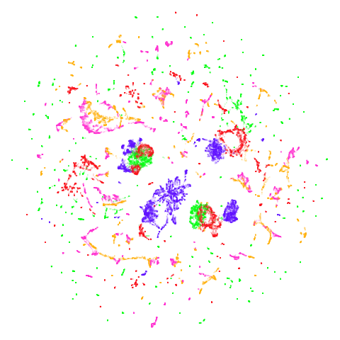
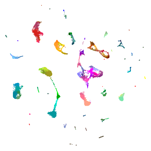
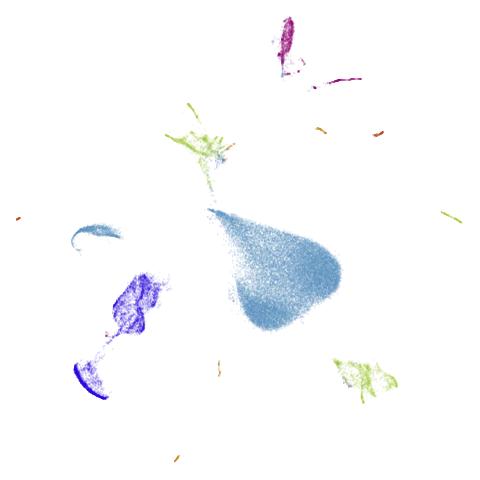
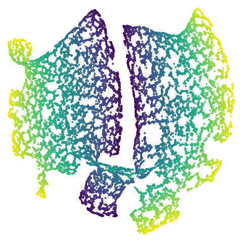
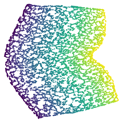
Below are some examples of using either the PCA initialization or a
spectral approach. On the first row, the left-hand image is the result
of using init = "pca", and the right-hand image is
init = "agspectral". On the second row, the left-hand image
is for init = "spectral". and the right-hand image is
init = "laplacian". Some datasets don’t have the second row
of images, because with the settings used here, they generate more than
one component in the graph, and therefore both
init = "spectral" and init = "laplacian" would
fall back to similar results as seen with init = "pca".
isoswiss
| pca | agspectral |
|---|---|
 |
 |
| spectral | laplacian |
|---|---|
 |
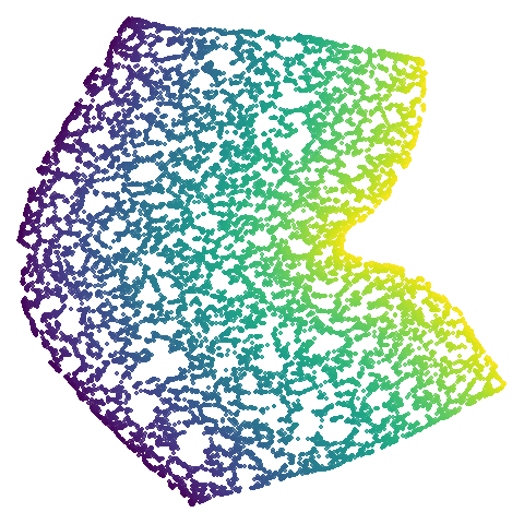 |
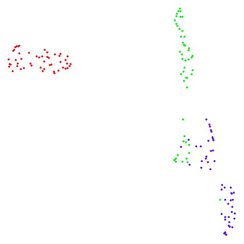
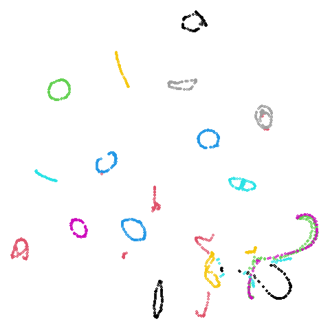
There are really only minor differences between the PCA results and the spectral results in most cases.
The big difference occurs with isoswiss. This shows the
Achilles heel of PCA for initialization: it does not have any respect
for manifolds. Where spectral initialization is able to “unfold” the
structure, PCA leaves it folded up and the projection onto 2D leaves it
broken up into three pieces.
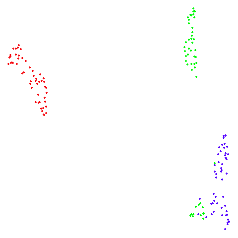
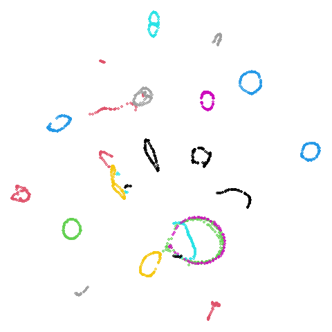
In most (but not all) cases, the agspectral results are
very similar to the spectral results. Again
isoswiss shows the limitations of the method. Like with
PCA, the manifold has not been initialized properly and some unpleasant
breakage occurs. There are certainly worse ways to initialize this
dataset though, as we shall see below. I don’t think the results here
are a fundamental limitation of the agspectral approach,
but the balance of the random vs near neighbor affinities may not be
ideal for this dataset.
The laplacian results also strongly resemble the
spectral initialization, and where they differ it’s not obvious to me if
one is strictly better than the other, so in terms of initialization for
UMAP, there doesn’t seem to be a strong advantage for using one type of
graph Laplacian over the other.
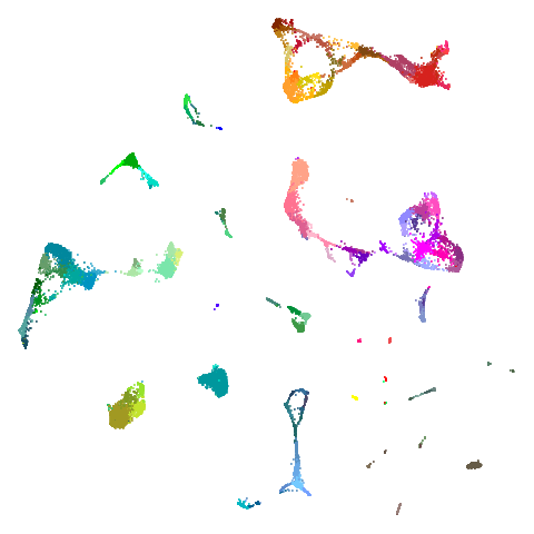
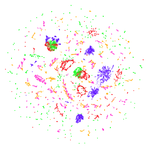
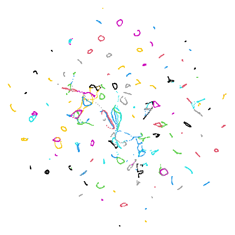
Random Initialization: rand
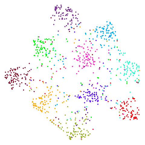
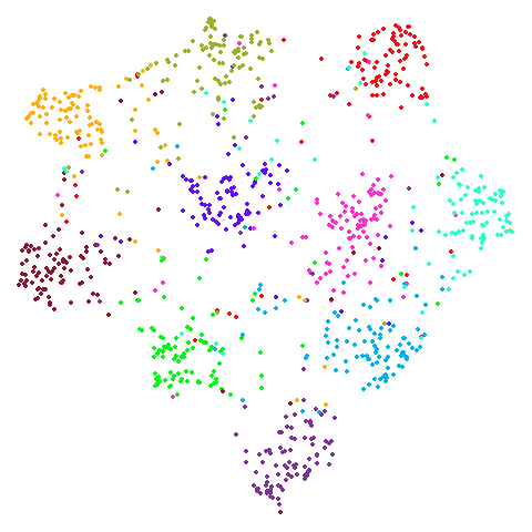
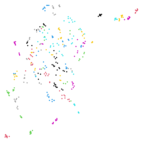
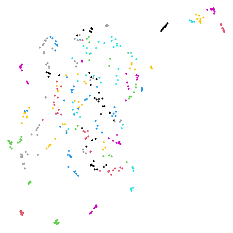
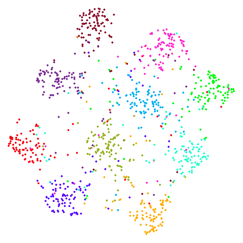
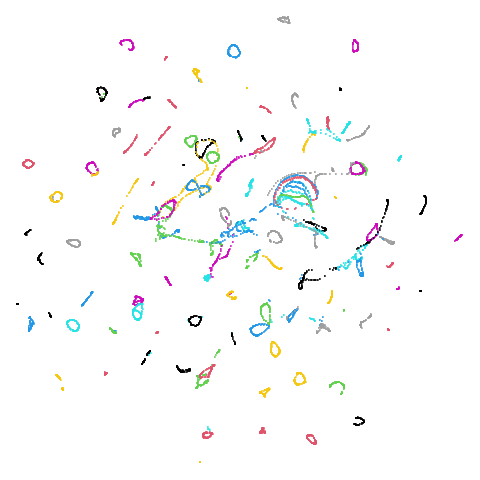
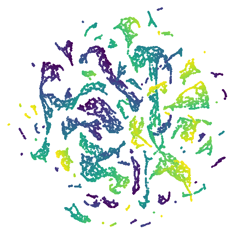
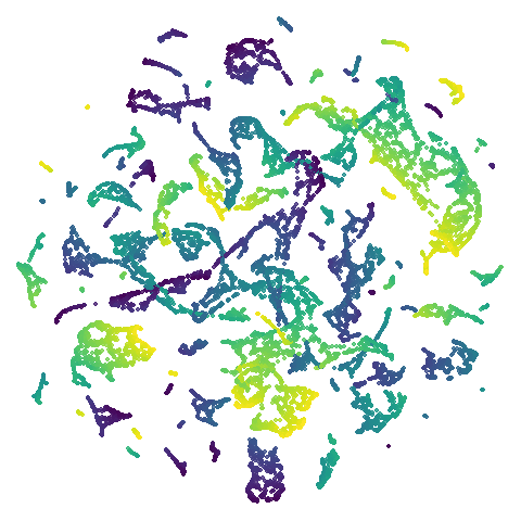
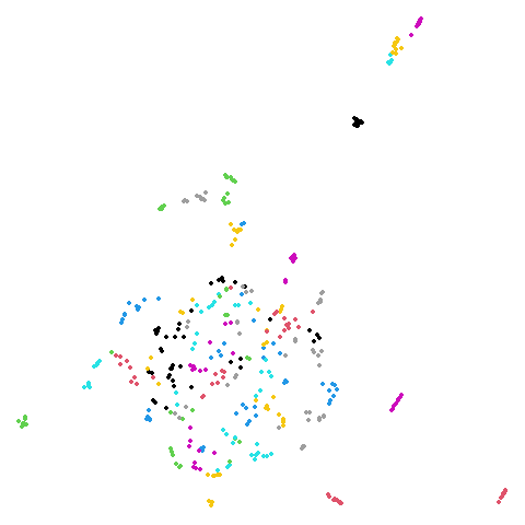
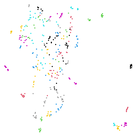
Below are two results each from using random initialization, so you can get a sense for how much variation you can expect from getting lucky or not with the initialization.
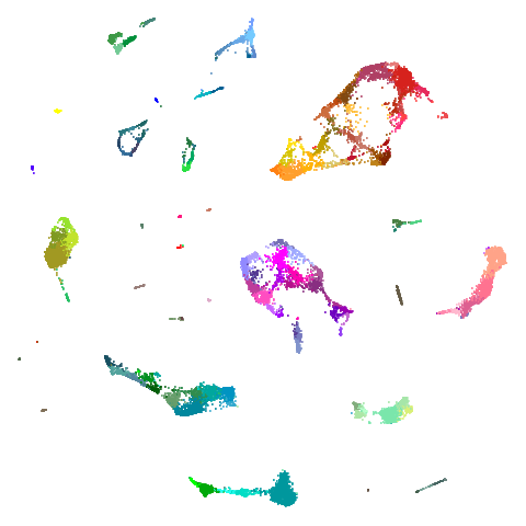
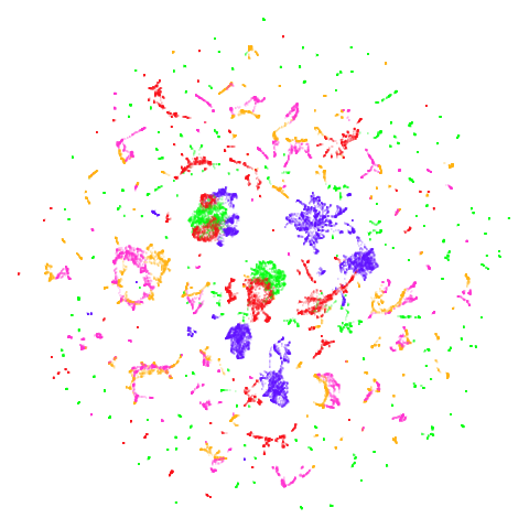
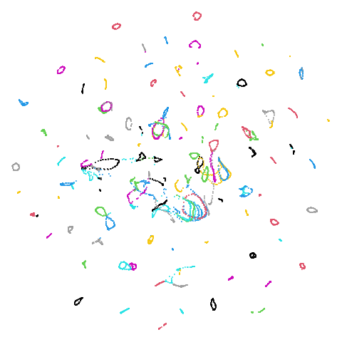
Random Initialization: lvrand
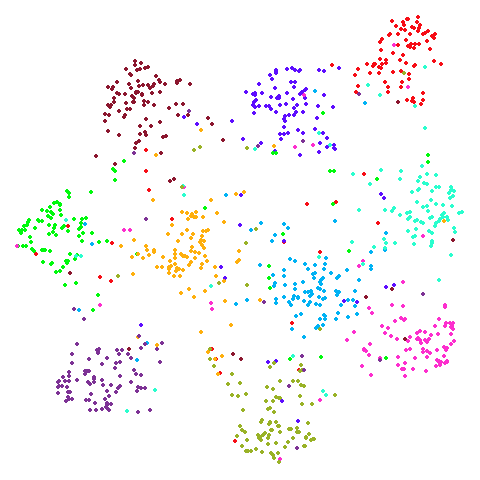
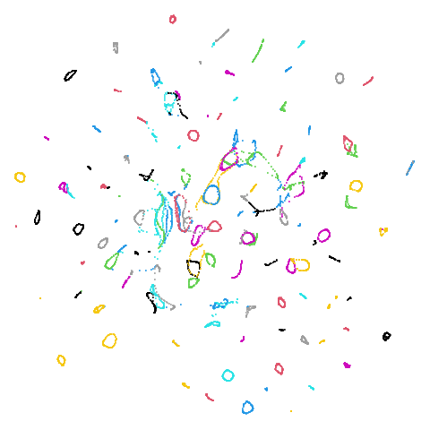
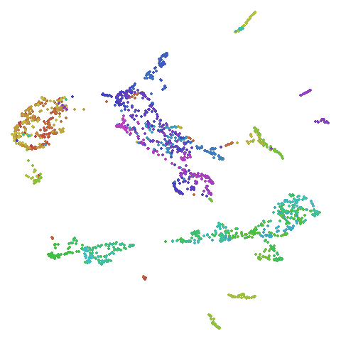
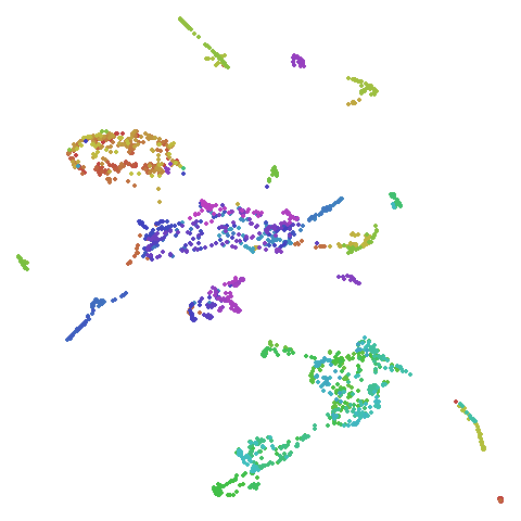
And here is the result of using random initialization in the t-SNE/LargeVis style, which use a Gaussian distribution over a much smaller initial range of coordinate values. Will it make much difference?
Recommendations
The default spectral initialization does a good job. If for some
reason you can’t use it, for example due to disconnections, then
init = "pca" is a good choice. The one exception is with
data where you think you have a manifold structure. In that case, you
would hope that you have a connected graph, in which case you won’t need
to use PCA.
I would love to say that agspectral can help you out if
you are having difficulty with a slow spectral initialization, and in
general it seems useful, but it may not work well with manifold data.
The laplacian initialization does not provide a meaningful
difference to the spectral initialization based on the results shown
here.
Random initialization should be used only as a last resort.
Increasing n_neighbors can sometimes help a bit, but you
may need to set it to a very high value (e.g. 150) and that may
introduce long-distance interactions that doesn’t represent your
data.
