umap2 is a new function that works a lot like
umap, but updates some defaults to make it easier to use,
and to bring it a bit more in line with the Python UMAP implementation.
The main differences are the following defaults:
-
min_dist = 0.1(and used to be0.01) It should always have had this value, I just messed up when I initially attempted to reproduce the default parameters from the Python UMAP package. -
init_sdev = "range". This scales the input coordinates between 0-10. I am pretty sure that this was introduced in the Python UMAP package after I wroteuwot, but we might as well follow suit. -
n_epochs = 500. Inumap(and Python UMAP) the default is 200 epochs unless the dataset is small (< 4,096 items). I think it’s better to just pick one default value, and withbatch = TRUE, you need slightly more epochs. -
batch = TRUE. This means use the Adam optimizer rather than the asynchronous stochastic gradient descent method. I find that in the vast majority of cases you get quite equivalent results, at the cost of needing a slightly larger value ofn_epochs, but that you get more consistent results when using multiple threads, so you can ameliorate the cost of the extra epochs by using more threads. -
n_sgd_threads, speaking of threads, if you go withbatch = TRUE, thenn_sgd_threadswill be set to the same number of threads that is used to find nearest neighbors and create the edge weights (controlled byn_threads). By default that’s the available number of threads divided by 2. Forumap, the defaultn_sgd_threadsis always 1 because of concerns around reproducibility. Note that even with a fixed seed and number of threads, the reproducibility concerns don’t fully go away withbatch = TRUEunless the nearest neighbor search is not subject to stochastic effects and usually it will be. - If you have RcppHNSW
installed, it will be used instead of Annoy. But bear in mind that the
only supported
metrics areeuclideanandcosine. - If you don’t RcppHNSW installed, but you do have rnndescent installed, that will be used instead of Annoy.
- If you use
rnndescentfor neighbors (whether because you have it installed and don’t haveRcppHNSWinstalled or because you have specified it withnn_method = "nndescent"), then you can use sparse matrices (of classdgCMatrix) as input (i.e. theXparameter). Inumapsparse matrix input is assumed to be a sparse distance matrix. As a result you cannot use sparse distance matrices as input toumap2but I very much doubt if anyone was using that feature, so this is a good trade-off. - If you set
a = 1, b = 1(and you don’t specifydens_scale), then the fastertumapgradient will be used.
These are not big changes so don’t expect large differences in
behavior, but I do strongly recommend installing (and loading)
RcppHNSW and rnndescent. I’ll use the MNIST
digits for a comparison. Use the snedata package from
github for this:
# install.packages("pak")
pak::pkg_install("jlmelville/snedata")

# or
# install.packages("devtools")
# devtools::install_github("jlmelville/snedata")
mnist <- snedata::download_mnist()Now let’s run umap and umap2 on the MNIST
data using their defaults.
Install RcppHNSW and rnndescent if you
haven’t already.
install.packages(c("RcppHNSW", "rnndescent"))With these libraries installed umap2 will use
RcppHNSW by default.
#install.packages(c("ggplot2", "Polychrome"))
library(ggplot2)
library(Polychrome)

set.seed(42)
palette <- as.vector(Polychrome::createPalette(
  length(levels(mnist$Label)) + 2,
  seedcolors = c("#ffffff", "#000000"),
  range = c(10, 90)
)[-(1:2)])
ggplot(
    data.frame(mnist_umap, Digit = mnist$Label),
    aes(x = X1, y = X2, color = Digit)
) +
    geom_point(alpha = 0.1, size = 0.5) +
    scale_color_manual(values = palette) +
    theme_minimal() +
    labs(
        title = "MNIST with uwot::umap",
        x = "",
        y = "",
        color = "Digit"
    ) +
    theme(legend.position = "right") +
    guides(color = guide_legend(override.aes = list(size = 5, alpha = 1)))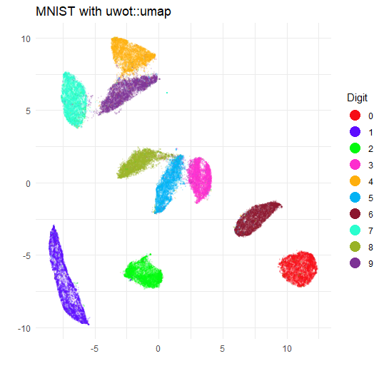
ggplot(
  data.frame(mnist_umap2, Digit = mnist$Label),
  aes(x = X1, y = X2, color = Digit)
) +
  geom_point(alpha = 0.5, size = 1.0) +
  scale_color_manual(values = palette) +
  theme_minimal() +
  labs(
    title = "MNIST with uwot::umap2",
    x = "",
    y = "",
    color = "Digit"
  ) +
  theme(legend.position = "right") +
  guides(color = guide_legend(override.aes = list(size = 5, alpha = 1)))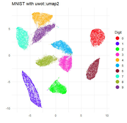
The biggest difference is that the clusters are somewhat larger and
closer together. This is due to the increase in min_dist.
If you re-run with min_dist = 0.01 you will get a plot that
is very similar to the umap plot.
I will spare you the ggplot2 incantation and go straight to the image:
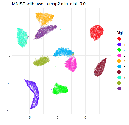
So there’s not much difference in whether you use umap2
or umap. In general, RcppHNSW and rnndescent can find
nearest neighbors at a given level of quality a bit faster than Annoy
does and even if you deviate from the default settings, you probably
have less to type with umap2 than umap.