Using rnndescent for nearest neighbors

This is a companion article to the HNSW article about how to use nearest neighbor data from other packages with uwot. You should read that article as well as the on uwot’s nearest neighbor format for proper details. I’m going to provide minimal commentary here.

The rnndescent package can be used as an alternative to the internal Annoy-based nearest neighbor method used by uwot. It is based on the Python package PyNNDescent and offers a wider range of metrics than other packages. See the supported metrics article in the rnndescent documentation for more details.

rnndescent can also work with sparse data. uwot is not yet directly compatible with sparse data input, but for an example of using rnndescent with sparse data see and then using that externally generated nearest neighbor data with uwot, see the sparse UMAP article. Here we will use typical dense data and the typical Euclidean distance.

First we need some data, which I will install via the snedata package from GitHub:

# install.packages("pak")
pak::pkg_install("jlmelville/snedata")

# or
# install.packages("devtools")
# devtools::install_github("jlmelville/snedata")

The HNSW article used the MNIST digits data, but to mix things up a bit I’ll use the Fashion MNIST data:

fashion <- snedata::download_fashion_mnist()
fashion_train <- head(fashion, 60000)
fashion_test <- tail(fashion, 10000)

This is structured just like the MNIST digits, but it uses images of 10 different classes of fashion items (e.g. trousers, dress, bag). The name of the item is in the Description column.

Installing rnndescent

Now install rnndescent from CRAN:

install.packages("rnndescent")
library(rnndescent)

UMAP with nndescent

library(uwot)

uwot can now use rnndescent for its nearest neighbor search if you set nn_method = "nndescent". The other settings are used to give reasonable results with batch mode (although feel free to change n_sgd_threads to however many threads you feel comfortable with your system using) and to return a model we can use to embed the test set data.

fashion_train_umap <-
  umap(
    X = fashion_train,
    nn_method = "nndescent",
    batch = TRUE,
    n_epochs = 500,
    n_sgd_threads = 6,
    ret_model = TRUE,
    verbose = TRUE
  )

UMAP embedding parameters a = 1.896 b = 0.8006
Converting dataframe to numerical matrix
Read 60000 rows and found 784 numeric columns
Using alt metric 'sqeuclidean' for 'euclidean'
Initializing neighbors using 'tree' method
Calculating rp tree k-nearest neighbors with k = 15 n_trees = 21 max leaf size = 15 margin = 'explicit' using 6 threads
Using euclidean margin calculation
0%   10   20   30   40   50   60   70   80   90   100%
[----|----|----|----|----|----|----|----|----|----]
***************************************************
Extracting leaf array from forest
Creating knn using 164273 leaves
0%   10   20   30   40   50   60   70   80   90   100%
[----|----|----|----|----|----|----|----|----|----]
***************************************************
Running nearest neighbor descent for 16 iterations using 6 threads
0%   10   20   30   40   50   60   70   80   90   100%
[----|----|----|----|----|----|----|----|----|----]
***************************************************
Convergence: c = 132 tol = 900
Finished
Keeping 1 best search trees using 6 threads
0%   10   20   30   40   50   60   70   80   90   100%
[----|----|----|----|----|----|----|----|----|----]
***************************************************
Min score: 2.41727
Max score: 2.4626
Mean score: 2.44337
Using alt metric 'sqeuclidean' for 'euclidean'
Converting graph to sparse format
Diversifying forward graph
Occlusion pruning with probability: 1
0%   10   20   30   40   50   60   70   80   90   100%
[----|----|----|----|----|----|----|----|----|----]
***************************************************
Diversifying reduced # edges from 840000 to 240155 (0.02333% to 0.006671% sparse)
Degree pruning reverse graph to max degree: 22
Degree pruning to max 22 reduced # edges from 240155 to 239741 (0.006671% to 0.006659% sparse)
Diversifying reverse graph
Occlusion pruning with probability: 1
0%   10   20   30   40   50   60   70   80   90   100%
[----|----|----|----|----|----|----|----|----|----]
***************************************************
Diversifying reduced # edges from 239741 to 214714 (0.006659% to 0.005964% sparse)
Merging diversified forward and reverse graph
Degree pruning merged graph to max degree: 22
Degree pruning to max 22 reduced # edges from 302918 to 302882 (0.008414% to 0.008413% sparse)
Finished preparing search graph
Commencing smooth kNN distance calibration using 8 threads with target n_neighbors = 15
Initializing from normalized Laplacian + noise (using irlba)
Commencing optimization for 500 epochs, with 1359492 positive edges using 8 threads
Using method 'umap'
Optimizing with Adam alpha = 1 beta1 = 0.5 beta2 = 0.9 eps = 1e-07
0%   10   20   30   40   50   60   70   80   90   100%
[----|----|----|----|----|----|----|----|----|----|
**************************************************|
Optimization finished

I will grant you that rnndescent has a lot to say for itself as it goes about its business. But you can always set verbose = FALSE.

Transforming test data

Now we have a UMAP model we can transform the test set data. Now notice that this looks exactly the same as the call we would make if we had used Annoy for nearest neighors: all the information needed for uwot to work out that it should use rnndescent for querying new neighbors is encapsulated in the fashion_train_umap model we generated.

fashion_test_umap <-
  umap_transform(
    X = fashion_test,
    model = fashion_train_umap,
    n_sgd_threads = 6,
    verbose = TRUE
  )

Read 10000 rows and found 784 numeric columns
Processing block 1 of 1
Reading metric data from forest
Using alt metric 'sqeuclidean' for 'euclidean'
Querying rp forest for k = 15 with caching using 6 threads
0%   10   20   30   40   50   60   70   80   90   100%
[----|----|----|----|----|----|----|----|----|----]
***************************************************
Finished
Searching nearest neighbor graph with epsilon = 0.1 and max_search_fraction = 1 using 6 threads
Graph contains missing data: filling with random neighbors
Finished random fill
0%   10   20   30   40   50   60   70   80   90   100%
[----|----|----|----|----|----|----|----|----|----]
***************************************************
min distance calculation = 0 (0.00%) of reference data
max distance calculation = 1810 (3.02%) of reference data
avg distance calculation = 172 (0.29%) of reference data
Finished
Commencing smooth kNN distance calibration using 6 threads with target n_neighbors = 15
Initializing by weighted average of neighbor coordinates using 6 threads
Commencing optimization for 167 epochs, with 150000 positive edges using 6 threads
Using method 'umap'
Optimizing with Adam alpha = 1 beta1 = 0.5 beta2 = 0.9 eps = 1e-07
0%   10   20   30   40   50   60   70   80   90   100%
[----|----|----|----|----|----|----|----|----|----|
**************************************************|
Finished

Again rnndescent is a lot chattier than when using Annoy.

Plotting the results

Now to take a look at the results, using ggplot2 for plotting, and Polychrome for a suitable categorical palette.

install.packages(c("ggplot2", "Polychrome"))
library(ggplot2)
library(Polychrome)

The following code creates a palette of 10 (hopefully) visually distinct colors which will map each point to the type of fashion item it represents. This is found in the Description factor column of the original data.

palette <- as.vector(Polychrome::createPalette(
  length(levels(fashion$Description)) + 2,
  seedcolors = c("#ffffff", "#000000"),
  range = c(10, 90)
)[-(1:2)])

And here are the results:

ggplot(
  data.frame(fashion_train_umap$embedding, Description = fashion_train$Description),
  aes(x = X1, y = X2, color = Description)
) +
  geom_point(alpha = 0.1, size = 1.0) +
  scale_color_manual(values = palette) +
  theme_minimal() +
  labs(
    title = "Fashion MNIST training set UMAP",
    x = "",
    y = "",
    color = "Description"
  ) +
  theme(legend.position = "right") +
  guides(color = guide_legend(override.aes = list(size = 5, alpha = 1)))

ggplot(
  data.frame(fashion_test_umap, Description = fashion_test$Description),
  aes(x = X1, y = X2, color = Description)
) +
  geom_point(alpha = 0.4, size = 1.0) +
  scale_color_manual(values = palette) +
  theme_minimal() +
  labs(
    title = "Fashion MNIST test set UMAP",
    x = "",
    y = "",
    color = "Description"
  ) +
  theme(legend.position = "right") +
  guides(color = guide_legend(override.aes = list(size = 5, alpha = 1)))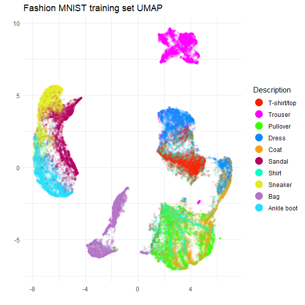

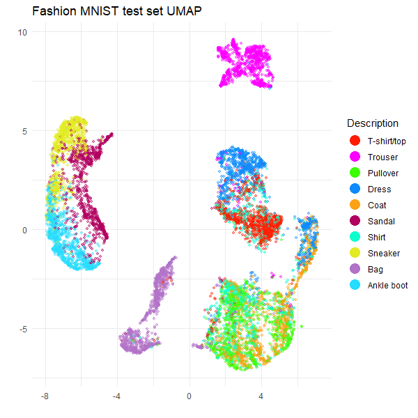
Fashion training data Fashion test set

These results are typical for Fashion MNIST result with UMAP. For example, see the first image in part of the Python UMAP documentation. So it looks like rnndescent with its default settings does a good job with this dataset.

A Minor Advantage of using `rnndescent`

If you use nn_method = "nndescent" then the UMAP model returned with ret_model = TRUE can be saved and loaded using the standard R functions saveRDS and readRDS. You don’t need to the use uwot-specific save_uwot and load_uwot, nor do you need to worry about unloading the model with unload_uwot, as you must with Annoy-based UMAP models. This is a consequence of rnndescent storing all its index-related data in pure R (no wrapping of existing C++ classes), but be aware that this can lead to much larger models on disk and in RAM.

Using `rnndescent` externally

If you want more control over the behavior of rnndescent then you can use it directly to create a nearest neighbor graph and then pass that result to the nn_method argument of umap. This isn’t usually necessary and if you do want more control I recommend using the nn_args argument of umap, which is a list of arguments to pass directly to rnndescent. If you decide to use rnndescent directly, the following section mainly uses default argument but demonstrates a workflow that can be customized for your own needs. The resulting UMAP plots will be essentially identical to those that are output when using nn_mmethod = "nndescent".

Build an index for the training data

First, we will build a search index using the training data. You should use as many threads (n_threads) as you feel comfortable with. You can also set verbose = TRUE, but when building an index you will see a lot of output so I won’t reproduce that here. The k parameter is the number of nearest neighbors that we are looking for. The index is tuned to work well for that number of neighbors. The metric parameter is the distance metric to use, but the default is Euclidean, so we don’t need to specify that. Finally, there is a stochastic aspect to the index building. You may get slightly different results from me, but I am leaving the seed unset so that we must both live with the inherently random nature of the index building process.

fashion_index <- rnnd_build(fashion_train, k = 15, n_threads = 6)

What’s in the returned index? A bunch of stuff:

names(fashion_index)

[1] "graph"           "prep"            "data"            "original_metric" "use_alt_metric"  "search_forest"   "search_graph"

Most of that is there to support searching the index. What we want is the graph. This is a list with two elements, idx and dist, which contain the nearest neighbor indices and distances respectively. The nearest neighbor of each item is itself, so we expect the first column of idx to be the sequence 1, 2, 3, … and the first column of dist to be all zeros.

fashion_index$graph$idx[1:3, 1:3]

     [,1]  [,2]  [,3]
[1,]    1 25720 27656
[2,]    2 42565 37551
[3,]    3 53514 35425

fashion_index$graph$dist[1:3, 1:3]

     [,1]      [,2]      [,3]
[1,]    0 1188.7826 1215.3440
[2,]    0 1048.0482 1068.3951
[3,]    0  532.6199  632.1653

With other nearest neighbor methods like HNSW and Annoy, you would have to run a separate query step to get the k-nearest neighbors for the data used to build the index. One of the advantages of rnndescent is that you can get this data directly from the index without the separate query step. Note that you can still query the index if you want to, and those results might be a bit more accurate, but I am quietly confident that the results from the index are sufficient for UMAP.

Query the test data

To get the test set neighbors, query the index with the test data:

fashion_test_query_neighbors <-
  rnnd_query(
    index = fashion_index,
    query = fashion_test,
    k = 15,
    n_threads = 6,
    verbose = TRUE
  )

fashion_test_query_neighbors$idx[1:3, 1:3]

      [,1]  [,2]  [,3]
[1,] 18095 53940 18353
[2,]  8573 31349  3885
[3,]   286 38144  3422

fashion_test_query_neighbors$dist[1:3, 1:3]

          [,1]      [,2]      [,3]
[1,]  482.2966  681.9905  708.4991
[2,] 1308.0019 1329.3134 1382.7317
[3,]  466.0322  538.5378  555.8795

As we are querying the test data against the training data, the nearest neighbor of any test item is not the test item itself.

We now have all the nearest neighbor data we need. The good news is that it’s already in a format that uwot can use so we can proceed straight to running UMAP.

Using rnndescent nearest neighbors with UMAP

UMAP on training data

To use pre-computed nearest neighbor data with uwot pass it as the nn_method parameter. In this case, that is the graph item in fashion_index. See the HSNW article for more details on the other parameters, but this is designed to give pretty typical UMAP results.

fashion_train_umap <-
  umap(
    X = NULL,
    nn_method = fashion_index$graph,
    batch = TRUE,
    n_epochs = 500,
    n_sgd_threads = 6,
    ret_model = TRUE,
    verbose = TRUE
  )

UMAP embedding parameters a = 1.896 b = 0.8006
Commencing smooth kNN distance calibration using 6 threads with target n_neighbors = 15
Initializing from normalized Laplacian + noise (using irlba)
Commencing optimization for 500 epochs, with 1359454 positive edges using 6 threads
Using method 'umap'
Optimizing with Adam alpha = 1 beta1 = 0.5 beta2 = 0.9 eps = 1e-07
0%   10   20   30   40   50   60   70   80   90   100%
[----|----|----|----|----|----|----|----|----|----|
**************************************************|
Optimization finished
Note: model requested with precomputed neighbors. For transforming new data, distance data must be provided separately

Transforming test data

Now we have a UMAP model we can transform the test set data. Once again we don’t need to pass in any test set data except the neighbors as nn_method:

fashion_test_umap <-
  umap_transform(
    X = NULL,
    model = fashion_train_umap,
    nn_method = fashion_test_query_neighbors,
    n_sgd_threads = 6,
    verbose = TRUE
  )

Read 10000 rows
Processing block 1 of 1
Commencing smooth kNN distance calibration using 6 threads with target n_neighbors = 15
Initializing by weighted average of neighbor coordinates using 6 threads
Commencing optimization for 167 epochs, with 150000 positive edges using 6 threads
Using method 'umap'
Optimizing with Adam alpha = 1 beta1 = 0.5 beta2 = 0.9 eps = 1e-07
0%   10   20   30   40   50   60   70   80   90   100%
[----|----|----|----|----|----|----|----|----|----|
**************************************************|
Finished

At this point you can plot the results, which will resemble those shown earlier.

A potentially simpler workflow

If you don’t want to transform new data, you can make life a bit easier. Instead of rnnd_build, use rnnd_knn which behaves a lot like rnnd_build but doesn’t preserve the index or do any index preparation. This saves time and the nearest neighbor results are returned directly in the return result. Let’s use the full Fashion MNIST results as an example:

fashion_knn <- rnnd_knn(fashion, k = 15, n_threads = 6)
names(fashion_knn)

[1] "idx"  "dist"

You can then pass fashion_knn to nn_method:

fashion_umap <-
  umap(
    X = NULL,
    nn_method = fashion_knn,
    batch = TRUE,
    n_epochs = 500,
    n_sgd_threads = 6,
    verbose = TRUE
  )

(I have spared you the log output). We don’t need to pass ret_model = TRUE here because we can’t transform new data. Here is the UMAP plot for the full Fashion MNIST dataset:

ggplot(
  data.frame(fashion_umap, Description = fashion$Description),
  aes(x = X1, y = X2, color = Description)
) +
  geom_point(alpha = 0.1, size = 1.0) +
  scale_color_manual(values = palette) +
  theme_minimal() +
  labs(
    title = "Fashion MNIST UMAP",
    x = "",
    y = "",
    color = "Description"
  ) +
  theme(legend.position = "right") +
  guides(color = guide_legend(override.aes = list(size = 5, alpha = 1)))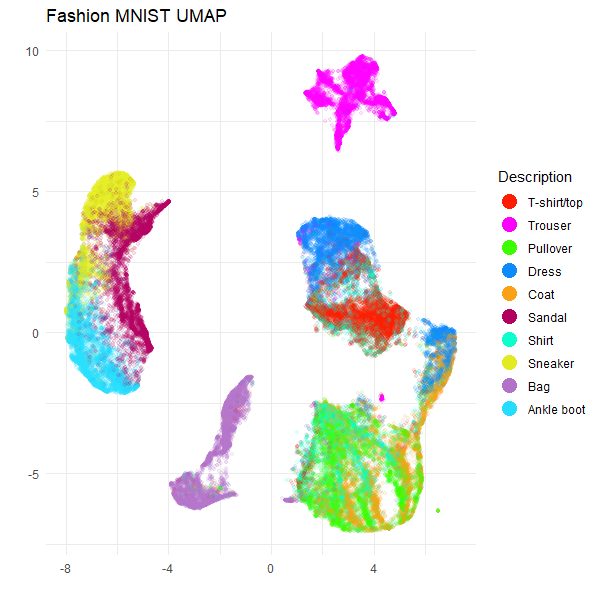

fashion UMAP

Everything looks as expected. However, if you think you might want to transform new data in the future, then you will need to completely restart the process, with rnnd_build and using ret_model = TRUE.

Conclusions

If you want to use rnndescent with uwot, then:

Install rnndescent and then use nn_method = "nndescent".

That handles most cases. If you want to use precomputed nearest neighbors, then:

Run rnndescent::rnnd_build on your training data.
Run uwot::umap with nn_method set to the graph item in the result of rnnd_build and remember to set ret_model = TRUE.

To transform new data:

Run rnndescent::rnnd_query on your test data, using the result of rnnd_build as the index parameter.
Run uwot::umap_transform with nn_method set to the result of rnnd_query.

If you don’t want to transform new data, then it’s even easier:

Run rnndescent::rnnd_knn on your training data.
Run uwot::umap with nn_method set to the result of rnnd_knn.

Installing rnndescent

UMAP with nndescent

Transforming test data

Plotting the results

A Minor Advantage of using rnndescent

Using rnndescent externally

Build an index for the training data

Query the test data

Using rnndescent nearest neighbors with UMAP

UMAP on training data

Transforming test data

A potentially simpler workflow

Conclusions

A Minor Advantage of using `rnndescent`

Using `rnndescent` externally