By default, uwot uses some conservative settings during
the stochastic gradient descent. But there are some options that can
speed things up:
-
n_sgd_threads = "auto"(or any value greater than one): this is the biggest thing you can do to speed up optimization. The optimization is now spread across multiple threads. The"auto"setting sets the value to that used in the other multi-threaded part of the code, which is controlled byn_threads. The downside to using multiple threads is that you can no longer guarantee the reproducibility of the results. Normally, you would expect the same results if you calledset.seedbefore each run. This will not be the case if setn_sgd_threads. -
pcg_rand = FALSE: the default random number generator used in the optimization is taken from the PCG family. This is quite fast and has good statistical properties. An alternative PRNG is an implementation of the Tausworthe “taus88” generator, which is used in the Python implementation of UMAP and which I have translated from Python into C++. By settingpcg_rand = FALSE, you will get the taus88 generator. This is faster than PCG, but bear in mind that PCG was designed by computer science professor Melissa O’Neill, and the taus88 implementation was translated into C++ by me (I am not a computer science professor), so if you have any concerns about the possibility of artifacts from bad random number generation, stick with PCG. Nonetheless, it probably gives results similar to that in the Python UMAP implementation most of the time. -
approx_pow = TRUE: the UMAP gradient requires some power calculations, which are quite slow compared to other arithmetic operations. An approximation to pow by Martin Ankerl can give a noticeable speed up. -
fast_sgd = TRUE: this just sets all three of the above options at once, to make life a bit easier.
If you need reproducibility (e.g. for scientific/publication
purposes), then using multiple optimization threads is a deal-breaker.
But for visualization purposes or if reproducibility isn’t that
important to you, then these settings can give a meaningful speed up of
the performance of uwot, without hurting the quality of the
layout.
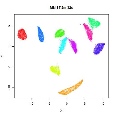
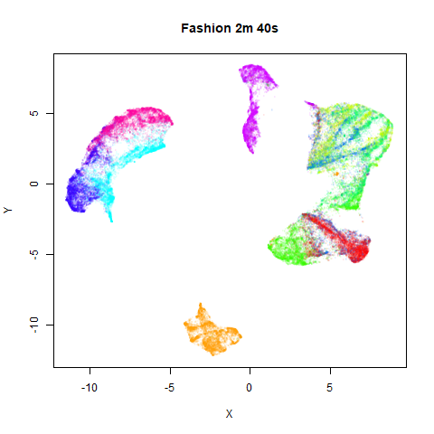
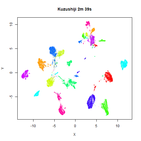
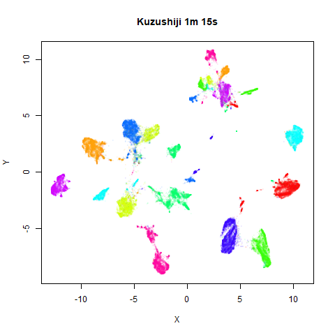
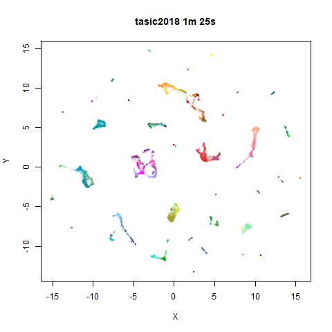
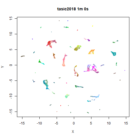
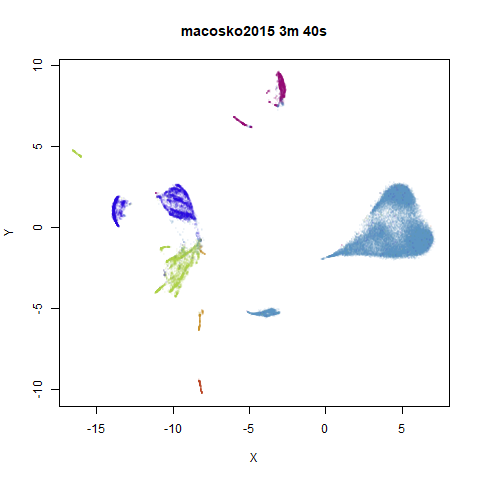
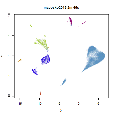
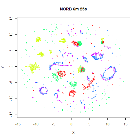
To prove it, here are some images of embeddings with the fast settings on and off. On the left are images with the optimization settings left in their default (slower) values. I also use PCA to reduce the dimensionality to 100:
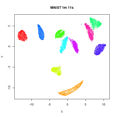
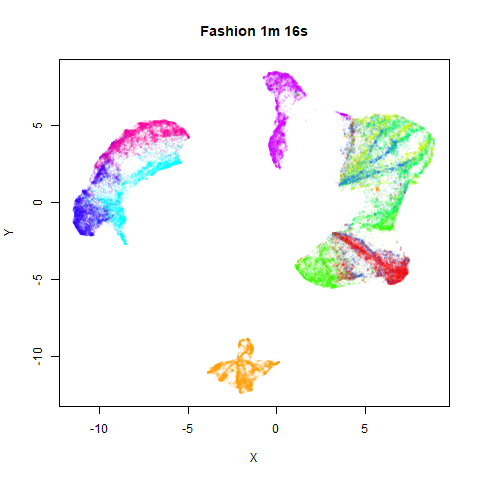
On the right are the embeddings from using
fast_sgd = TRUE:
Six threads were used in the stochastic gradient descent.
For details on the datasets, see the examples
page. The timings are given in the title, in minutes and seconds. Note
that this is for entire run, not just the optimization phase, i.e. it
includes the PCA dimensionality reduction and nearest neighbor search,
which is usually the slowest part of the run and which is not affected
by fast_sgd.
norb
 |
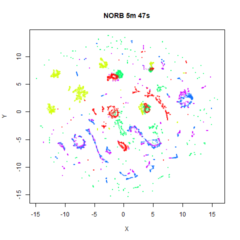 |
The distribution of clusters here does a look a little bit different,
but I think it’s within the variation that one would expect from the
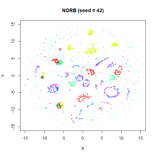
stochastic nature of the optimization. To bolster my point, here are two
further runs of UMAP on the NORB dataset with
fast_sgd = FALSE and different seeds:
 |
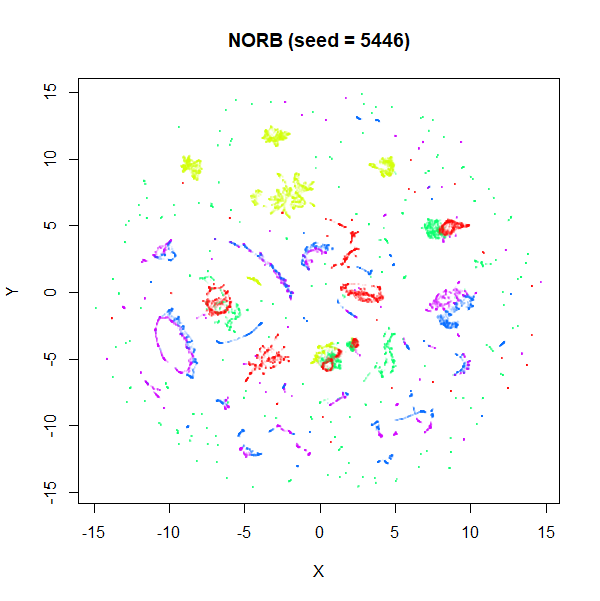 |
I think if you didn’t know one of these four images was generated
with the fast settiings, you’d be hard pressed to pick it out of the
line up. The variation between images is more likely due to the default
n_neighbors being too low to capture the global structure.
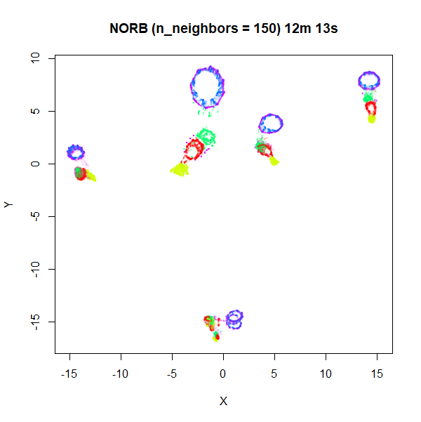
Here’s some plots with n_neighbors = 150, and
n_epochs = 500 to account for the increased number of edges
that need sampling:
 |
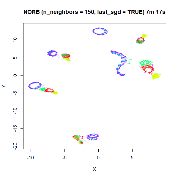 |
Apart from one of the blue loops being open in the
fast_sgd = TRUE result, which is probably fixable with a
longer optimization, the global arrangement of the two plots is pretty
similar.
Recommendations
From these results, I’d say that the fast_sgd = TRUE
settings give results which are effectively indistinguishable from the
slower settings, so if you want to save a bit of time, there seems no
harm in using them. The actual time savings you’ll see depend on how
long the nearest neighbor search takes, and any initial PCA you carry
out on the input (as we do in all these examples) can take a fair amount
of the run time. For example on NORB, the PCA takes up 5 minutes of the
six-and-a-half minute total run time, so there’s not a lot of time to be
saved. But for MNIST and Fashion, you can effectively halve the run time
(with six threads, anyway).
If reproducibility is important to you, then using multiple threads
in the optimization is out of the question, although that’s what gives
the biggest speed increase. However, you could still consider setting
approx_pow = TRUE, pcg_rand = FALSE. For MNIST-sized
datasets (mnist, fashion,
kuzushiji) I saw a reasonable speed up of around 25%. For
datasets where the PCA and nearest neighbor search dominates, the gains
are smaller: a 10-15% speedup for tasic2018 and
macosko2015, and only 5% for norb. If you need
to set n_epochs higher, then these time savings will
increase.
Update December 22 2024
Since I wrote this document, there are some extra options available.
As of uwot 0.2.3, the rng_type parameter is preferred over
pcg_rand. The equivalent of pcg_rand = FALSE
is rng_type = "tausworthe", but you can also set
rng_type = "deterministic", which will deterministically
sample the vertices. This can give a bigger speed up than
rng_type = "tausworthe".
Further, if you are using the umap2 function and have rnndescent
installed, the following parameters can be used to speed up the nearest
neighbor search:
nn_method = "nndescent", nn_args = list(n_trees = 8, max_candidates = 20).
Finally, you can also consider setting
negative_sample_rate = 4, which will give a slight speed up
versus the default sample rate of 5.
These suggestions are based on a comment by Leland McInnes on Reddit.
