UMAP on some simple datasets

The distill publication How to Use t-SNE Effectively provides some interactive examples of t-SNE on a variety of simple datasets and demonstrates the effect of changing its hyperparameters, mainly the perplexity, which acts like a continuous version of the n_neighbors parameter in UMAP.

Below, I will repeat some results using UMAP instead of t-SNE, which might highlight some differences between the two methods. Sadly, there won’t be any fancy in-browser interactive demos.

The datasets used in the distill publication are available translated to R in the snedata package.

UMAP results are all run with the n_neighbors parameter set to match the perplexity used in t-SNE all other parameters left at their default values. There are two minor exceptions: in UMAP, a point is a neighbor of itself, which isn’t the case with perplexity. This doesn’t make much difference for large perplexities, but for the low perplexity values of 2 and 5, I use n_neighbors = 3 and n_neighbors = 6, respectively.

I won’t repeat the t-SNE results here. You should refer back to the distill page to compare. I have kept the same order of datasets and used the same colors so it should be straightforward to keep things tracked.

Grid

A 2D grid with regularly spaced points.

grid2d <- snedata::grid_data(n = 20)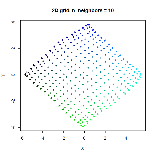

Like t-SNE, UMAP tends to expand denser regions of data, so there is a bigger gap between points in the middle of the grid.

2 Clusters

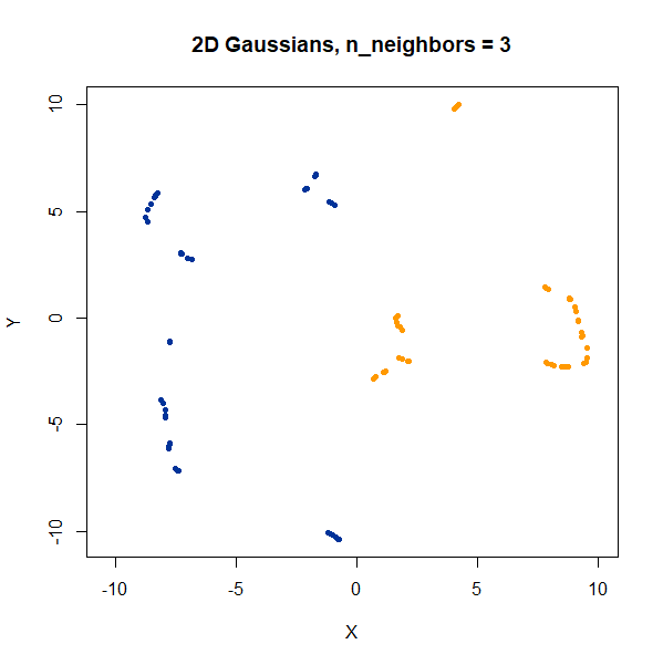
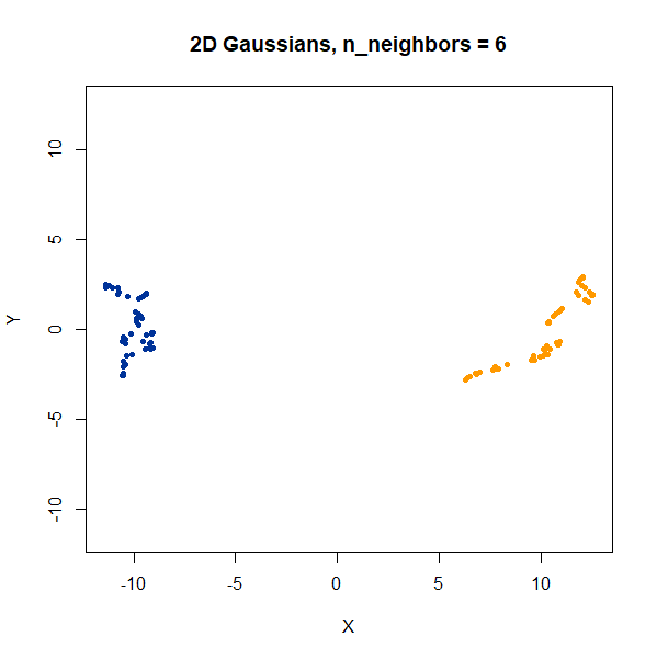
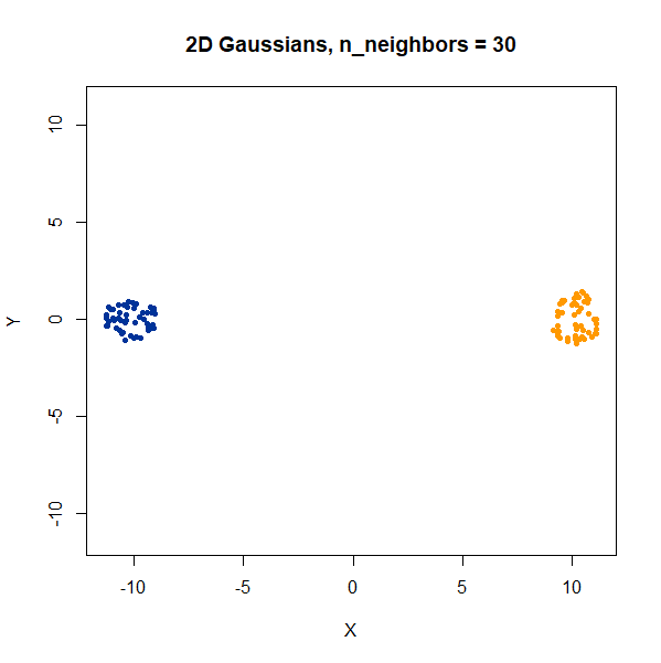
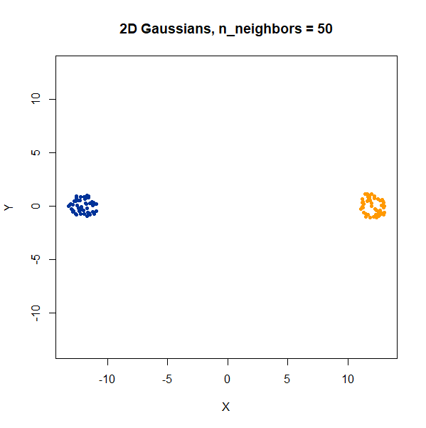
Two 2D Gaussian clusters of equal variance, and 50 points each.

gauss2d <- snedata::two_clusters_data(n = 50, dim = 2)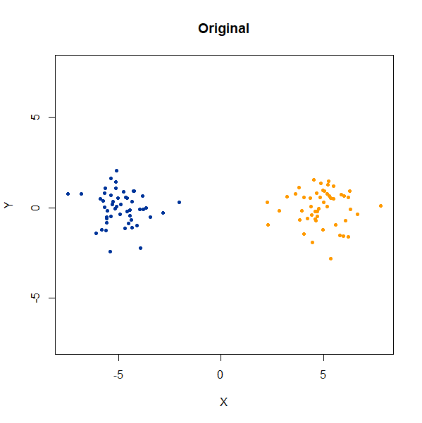

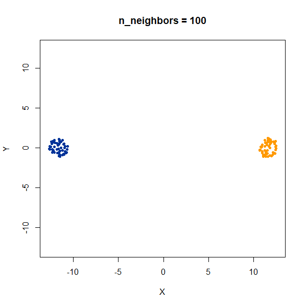Setting n_neighbors too low clearly gives results which are too local.

Cluster Densities

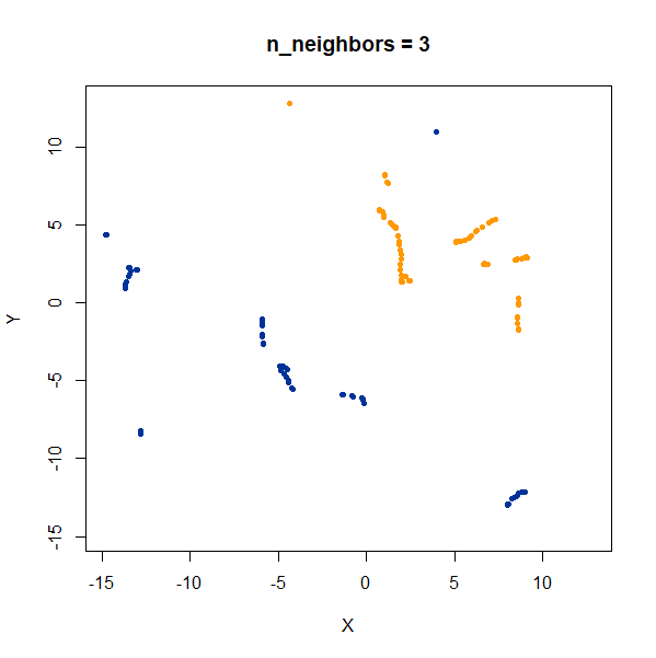
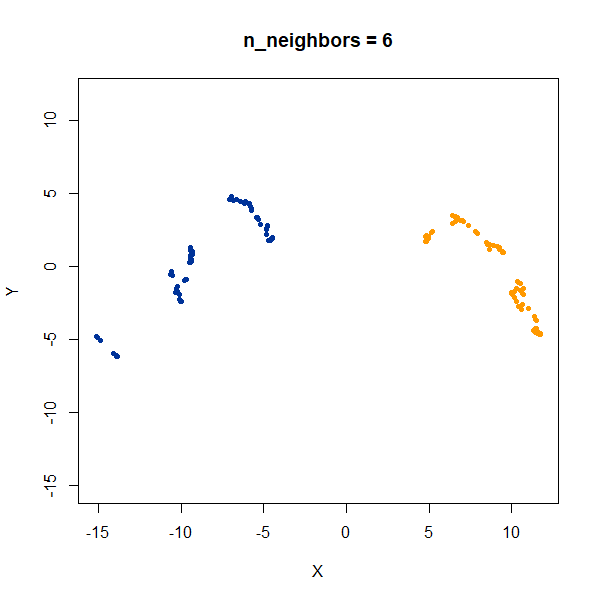
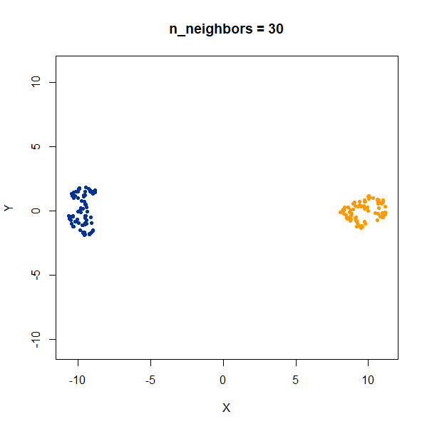
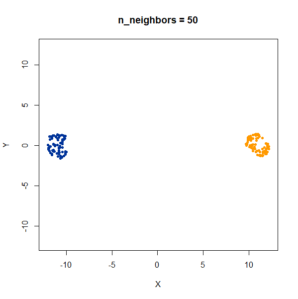
In this example, one of the clusters (the yellow one) is much denser (and hence smaller) than the other.

gauss2d_scale <- snedata::two_different_clusters_data(n = 75, scale = 10, dim = 2)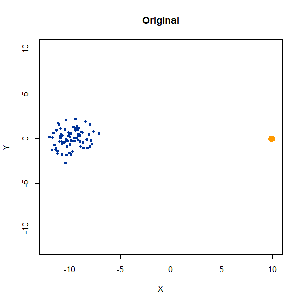

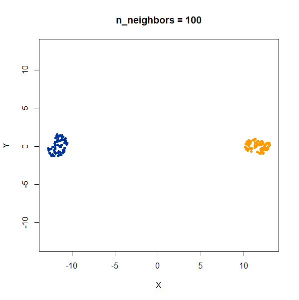Again like t-SNE, UMAP does not reproduce the relative cluster densities.

Cluster Size

x100a <- snedata::gaussian_data(n = 100, dim = 50, color = "blue")
x1000b <- snedata::gaussian_data(n = 1000, dim = 50, color = "orange")
x1000b[, 1:50] <- x1000b[, 1:50] <- x1000b[, 1:50] + 10
x200 <- rbind(x100a, x100b)
x1100 <- rbind(x100a, x1000b)

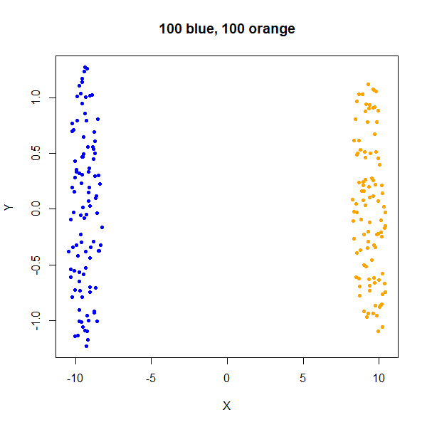
As an aside, what about two clusters with the same density but different numbers of points? Below is an example with two clusters with equal sizes (100 points each), and then where the orange cluster contains 1000 points:

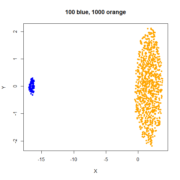From this example you can see that UMAP will display clusters with more members as being larger. This can have implications for the visualization if you have a minority class that you are most interested in.

Distances Between Clusters

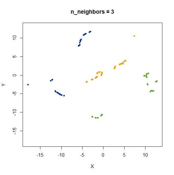
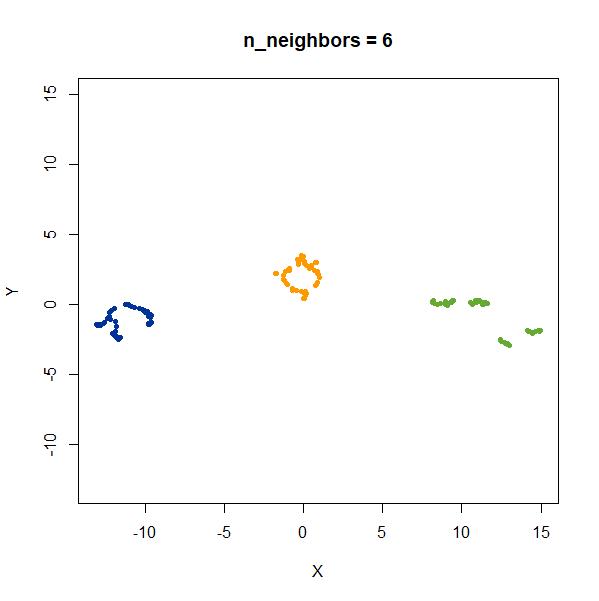
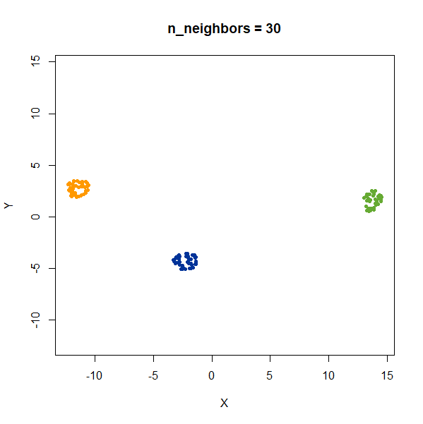
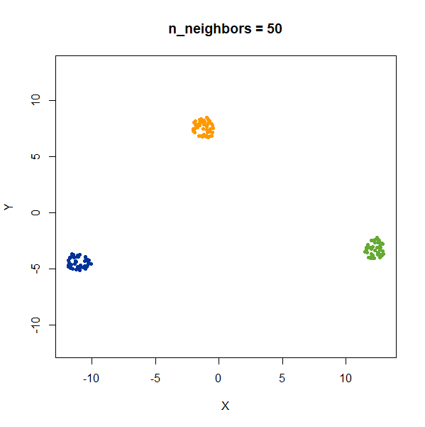
In this example, we are back to gaussians with the same variances, but now one of them (the green one) is much further away than the other two.

gauss_3clusters <- snedata::three_clusters_data(n = 50, dim = 2)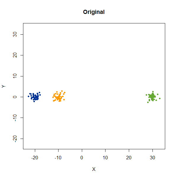

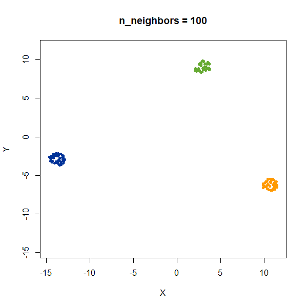There’s not really any value of n_neighbors where the correct relative distances are reproduced. On the other hand, at least we don’t see any strange distortion of the size of the green cluster at high values for n_neighbors, where as the t-SNE results start showing distortions at high perplexity.

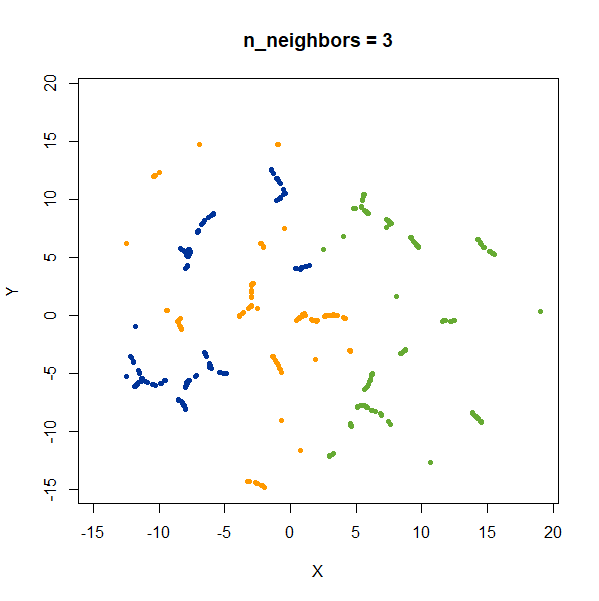
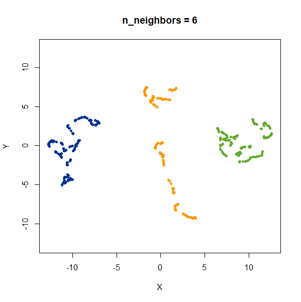
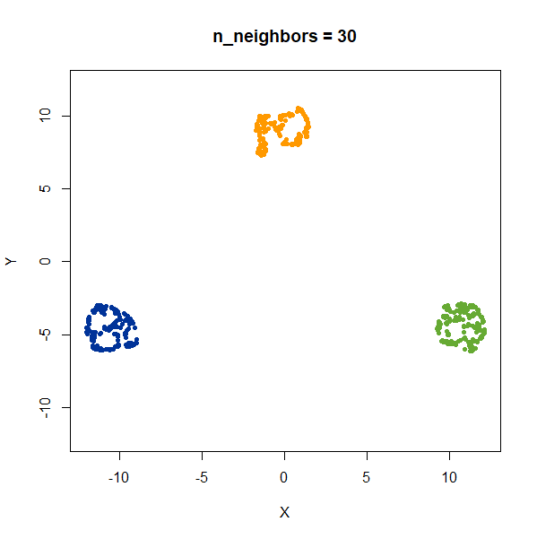
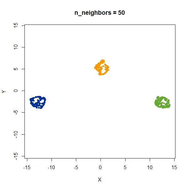
We then repeat with a larger number of points in each cluster:

gauss_3clusters200 <- snedata::three_clusters_data(n = 200, dim = 2)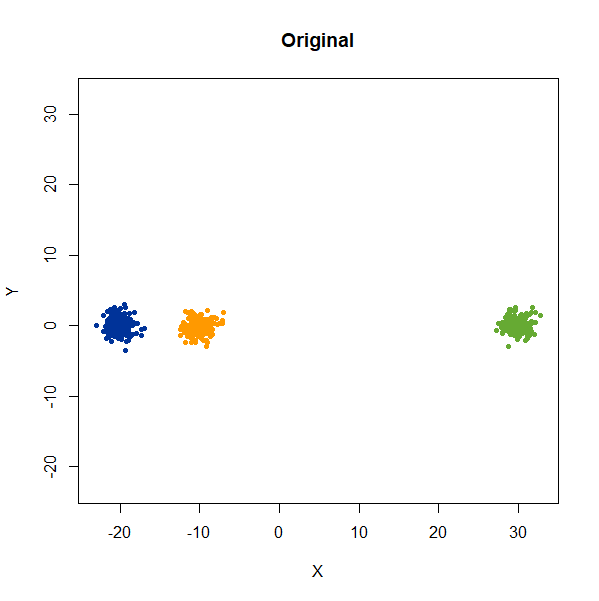

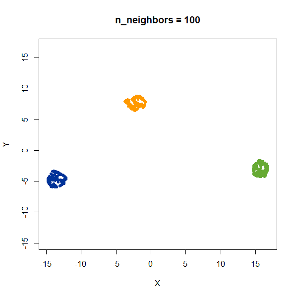Results are very consistent with a sensible value of n_neighbors, but it’s clear that UMAP does not reproduce relative distances in this case.

Random Noise

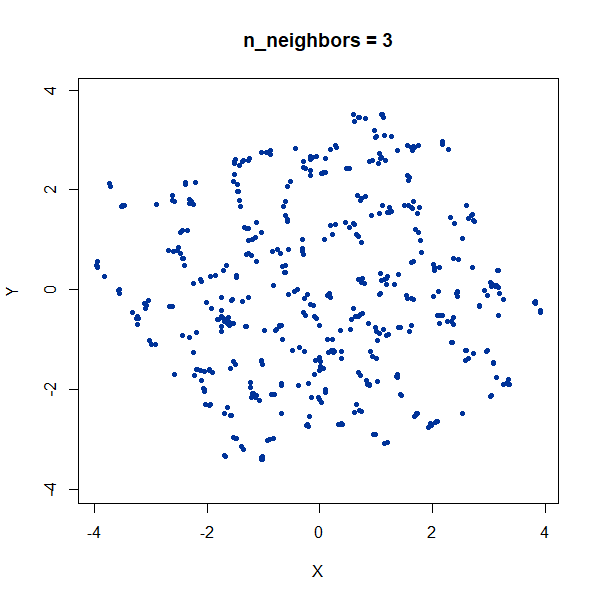
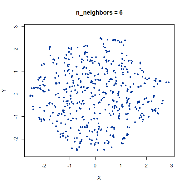
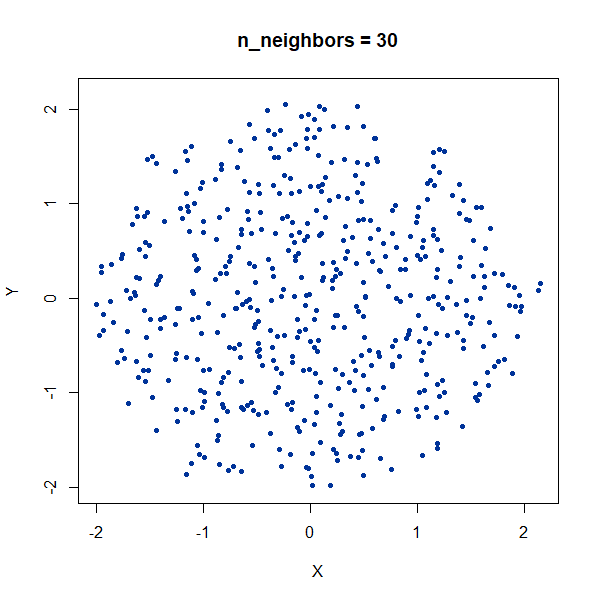
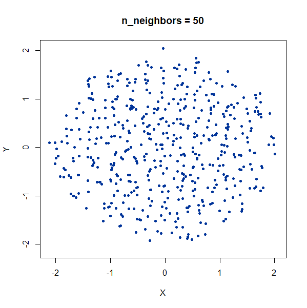
A single high-dimensional Guassian:

gauss100d <- snedata::gaussian_data(n = 500, dim = 100, color = "#003399")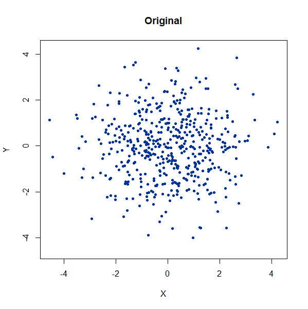

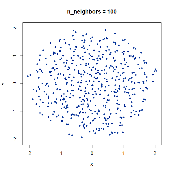Again, we see t-SNE-like behavior: the density of points in the projection is more even than the linear projection provided by PCA. It’s also clear that low values of n_neighbors could mislead you into seeing large numbers of small clusters that aren’t really there.

Elongated Shapes

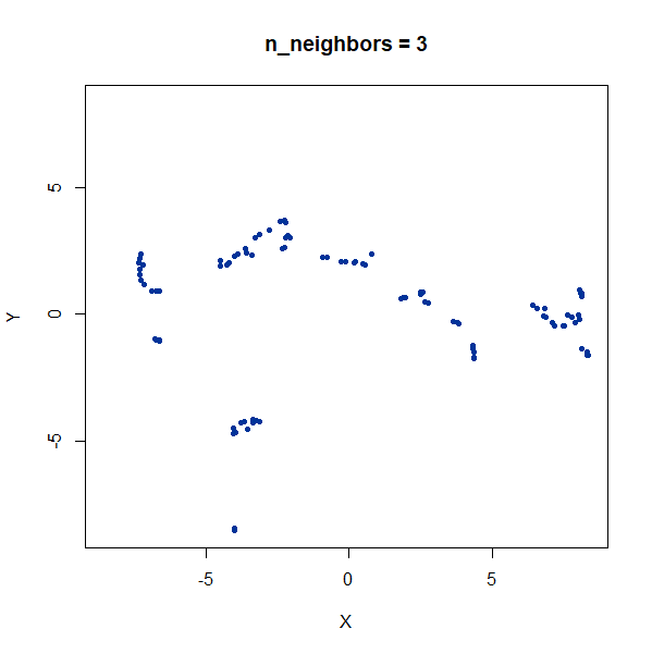
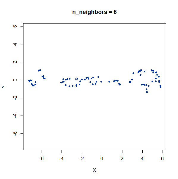
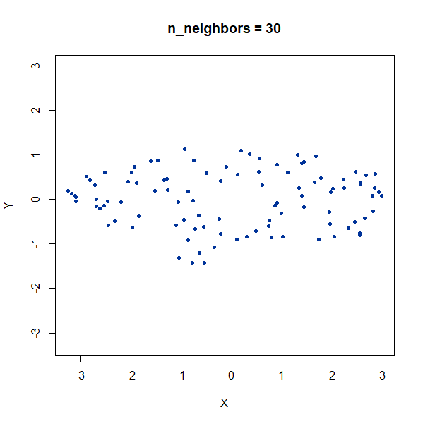
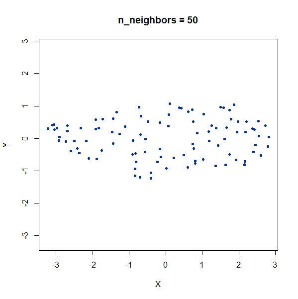
An ellipsoidal cluster:

gauss_long <- snedata::long_gaussian_data(n = 100, dim = 50, color = "#003399")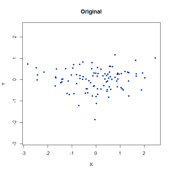

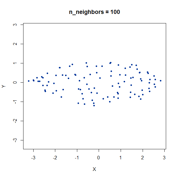Once again, UMAP behaves pretty well here as long as n_neighbors is sufficiently high.

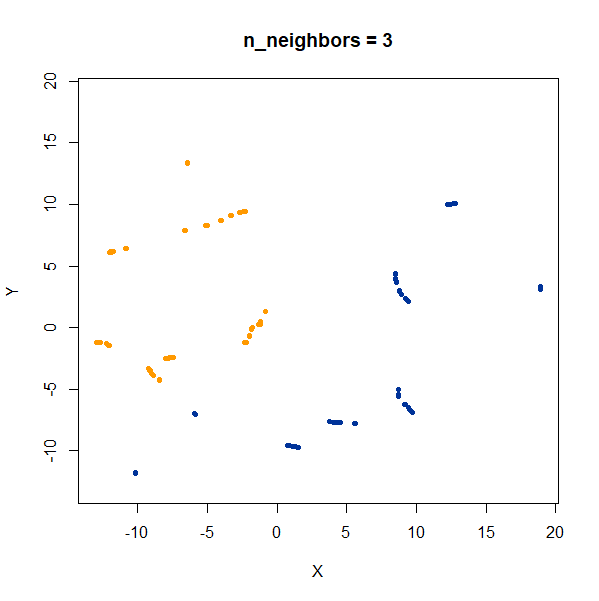
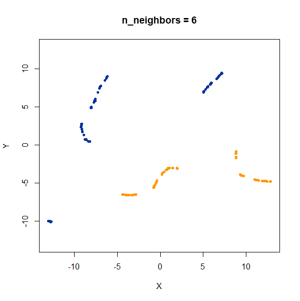
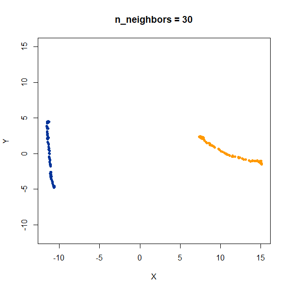
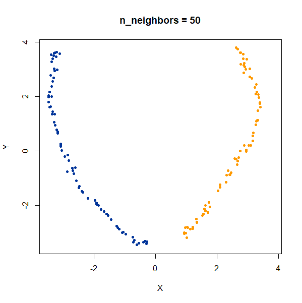
Now, here are two ellipsoidal clusters:

gauss_2long <- snedata::long_cluster_data(n = 75)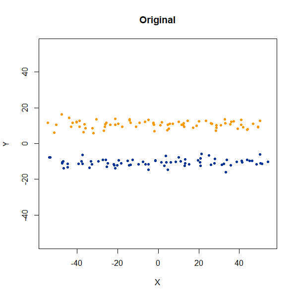

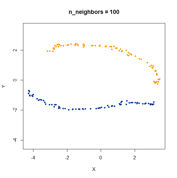The density distortion effect is also apparent here, causing the clusters to curve.

Topology

Containment

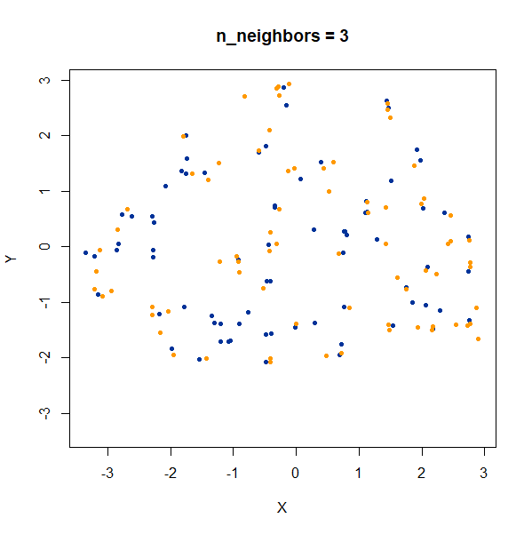
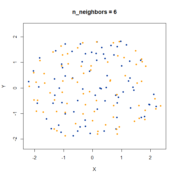
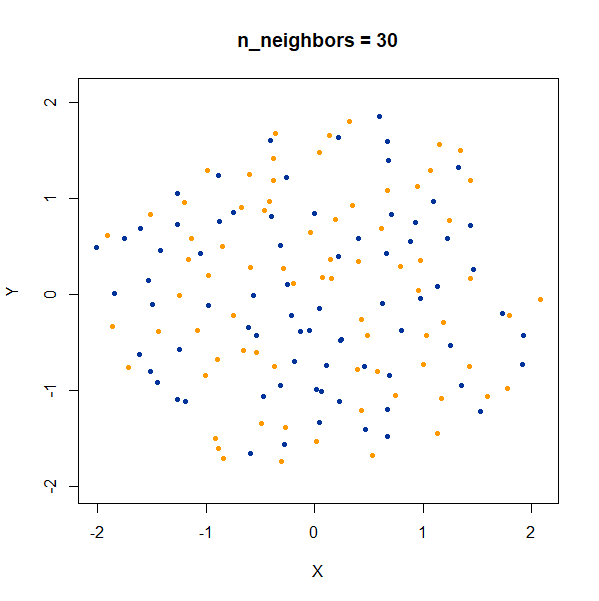
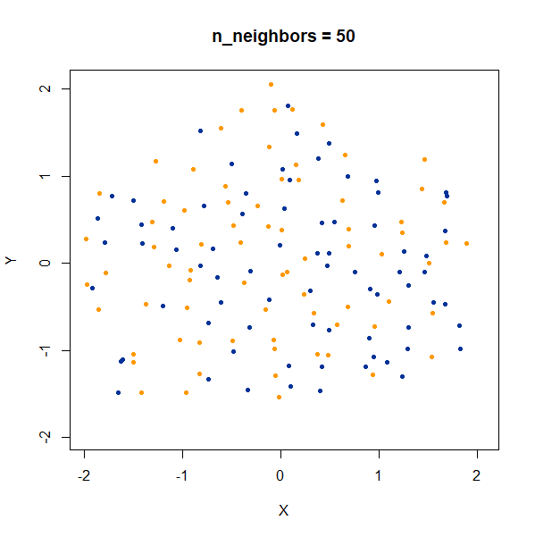
In this dataset, there are two 50D gaussian clusters, centered over the same location, but as the PCA plot on the top left row shows, the blue cluster has a much smaller variance and so is “contained” inside the yellow cluster.

subset50d <- snedata::subset_clusters_data(n = 75, dim = 50)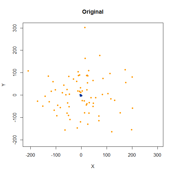

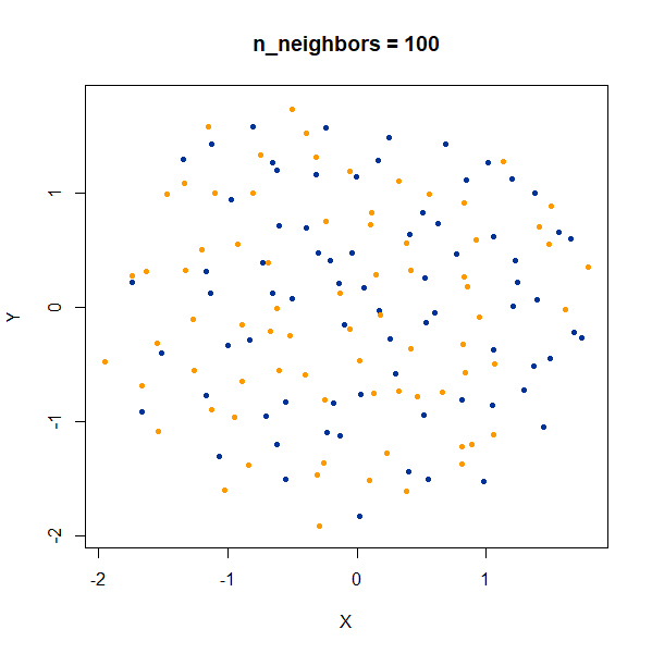At last a difference with the t-SNE results. With t-SNE, the containment relationship can be displayed with a suitable choice of perplexity, at the cost of the yellow cluster gaining a more ring-like shape. UMAP, however, stubbornly refuses to show anything of the sort, with the blue cluster expanded to overlap the yellow cluster even at the higher values of n_neighbors.

Linked Rings

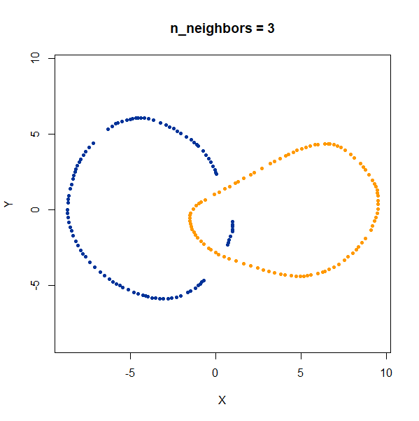
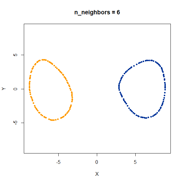
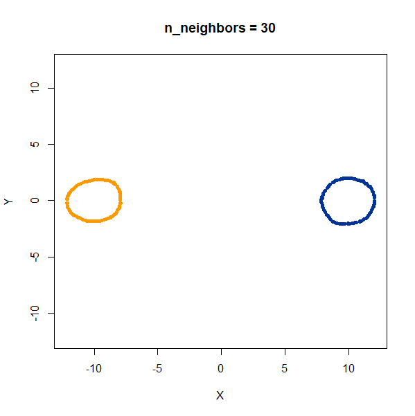
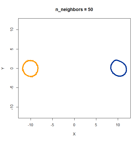
2D linked rings, embedding into 3D (one is at right angles to the other).

linked_rings <- snedata::link_data(n = 100)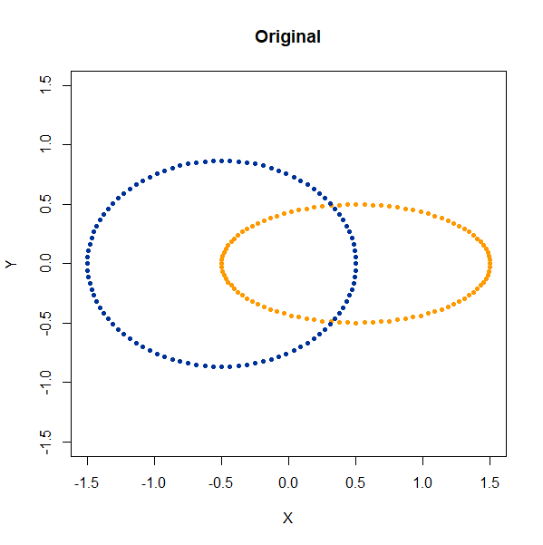

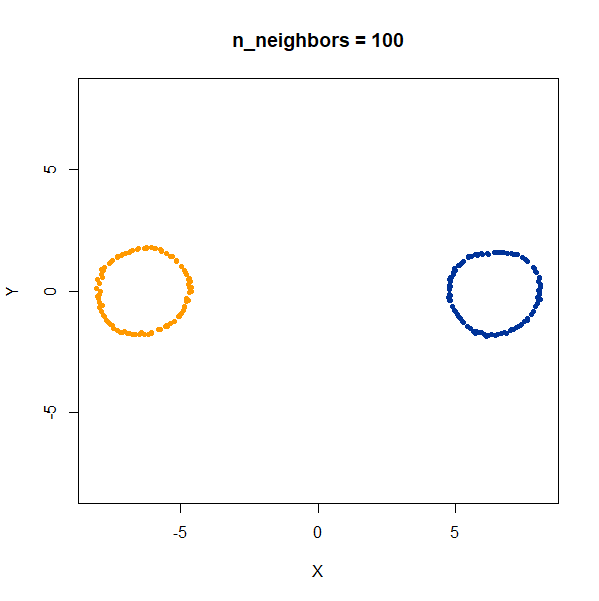The t-SNE results show the rings between separate at low perplexity, and only linked at high perplexities. The UMAP results are always unlinked except at a very low value of n_neighbors, and even then this seems to be an artifact of the number of epochs and the random seed. If you set n_epochs higher, then the rings will be invariably unlinked.

Trefoil Knot

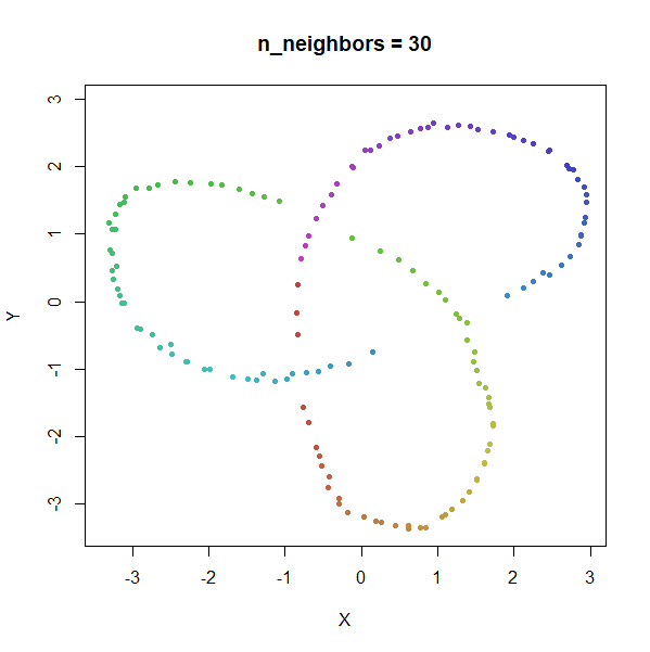
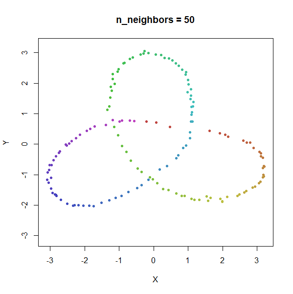
trefoil <- snedata::trefoil_data(n = 150)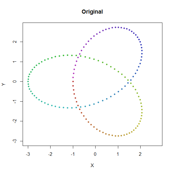

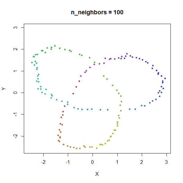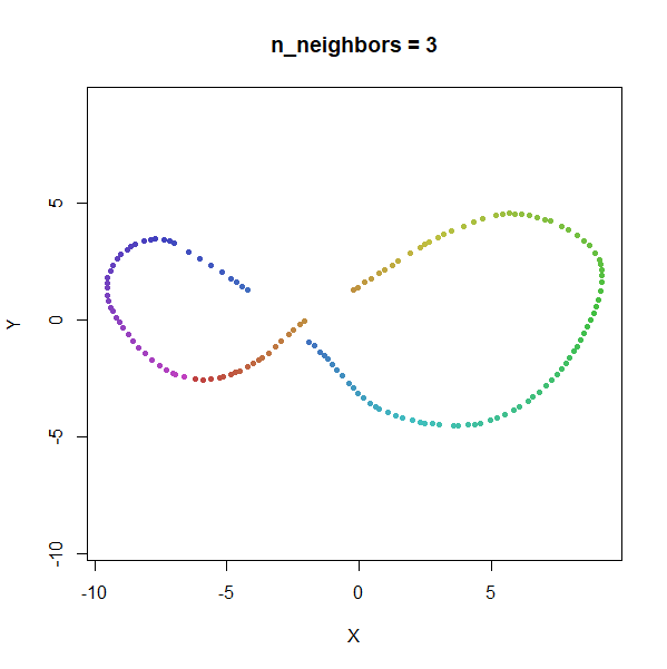
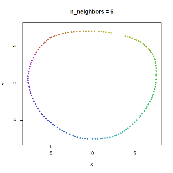
Results here are quite similar to the t-SNE results. At low values of n_neighbors, the knot is unfolded into a circle, and at higher values, the folded form appears. As with the linked rings, the results you get at low values of n_neighbors are more consistent at higher values of n_epochs.

What are we to make of all this? Mainly, that the UMAP results are a bit more consistent than that of t-SNE, in the sense that changing n_neighbors doesn’t lead to very different results in the way that changing perplexity does for t-SNE, although these effects are mainly restricted to the three cluster and the containment example. You may see this as an advantage to t-SNE. Personally, I am a bit skeptical that you would see this sort of thing in real world datasets.

It’s also worth noting that, like t-SNE:

• Inter-cluster distances are not reproduced.
• Relative cluster sizes are not reproduced.
• Denser regions of space are expanded more than less dense parts.