LargeVis

April 19, 2020

This article retains its original experiments and examples. For current package usage, see the usage guide.

LargeVis (paper and github repo) is a clever method that allows a t-SNE like visualization using stochastic gradient descent, which scales much better than the Barnes-Hut approximation to t-SNE. LargeVis does not minimize the same cost function as t-SNE, but it is similar. There is an R package that is sadly no longer on CRAN, but can be installed from github easily enough. The lvish function that is part of uwot is close enough to the real LargeVis for my purposes. Both of these packages replicate the stochastic gradient descent approach to optimization, which is the point of the method: to be scalable to large datasets. As a result, I’m not aware of other code that has implemented the LargeVis method in an exact gradient form.

Theory

The theory of LargeVis is covered in plenty of depth over on the theory page. Here’s a summary. An exact gradient cost function looks like:

C_{\mathrm{LV}} = -\sum_{ij} p_{ij} \log w_{ij} -\gamma \sum_{ij} \log \left( 1 - w_{ij} \right)

where p_{ij} are input probabilities generated in the same way as t-SNE (perplexity, averaging, normalization) and w_{ij} are output weights, also defined in the same way as t-SNE. \gamma is weight factor for the repulsive contributions. This is something that needs to be experimented with. The default value in the SGD implementation (\gamma = 7) is way too large once you start considering all pairs of points.

The gradient with respect to the output coordinates, \mathbf{y} is:

\frac{\partial C_{\mathrm{LV}}}{\partial \mathbf{y}_i} = 4\sum_j^N \left[ \frac{p_{ij}}{ 1 + d_{ij}^2 } -\frac{\gamma }{ \left( \epsilon + d_{ij}^2 \right) \left( 1 + d_{ij}^2 \right) } \right] \left(\mathbf{y}_i - \mathbf{y}_j\right)

where d_{ij} is the Euclidean output distance between coordinates. \epsilon is a small positive value chosen to prevent division by zero. In the LargeVis source code, it’s set to 0.1.

In an email discussion, Dmitry Kobak made the clever observation that if you set \epsilon = 1 (practically that’s not a small value so you probably shouldn’t do this, but bear with us), and you can write the gradient as:

\frac{\partial C_{\mathrm{LV}}}{\partial \mathbf{y}_i} = \frac{4}{N}\sum_j^N \left( v_{ij} - N\gamma w_{ij} \right) w_{ij} \left(\mathbf{y}_i - \mathbf{y}_j\right)

I have also used the substitution p_{ij} = v_{ij} / N. This expression resembles other methods’ gradients quite closely:

• t-distributed Elastic Embedding, where the t-EE parameter \lambda = N\gamma.
• if you choose \gamma = 1/Z at each iteration (where Z = \sum w_{ij}), you get the t-SNE gradient.

Un-normalized LargeVis

Does it make sense to be matching p_{ij} to w_{ij} in the cost function, rather than v_{ij}? As it happens, the LargeVis source code doesn’t actually generate the p_{ij} from the v_{ij}. It doesn’t need to, because the absolute values aren’t needed in the stochastic gradient descent method it uses: the relative values are used to generate the probability of sampling a point, and that is unaffected by scaling by N or not. In the gradient calculation, p_{ij} is set to 1, as the magnitude of the attractive force has already been accounted for by how often it’s sampled.

If we replace p_{ij} with v_{ij} to create an un-normalized LargeVis, the gradient is now:

\frac{\partial C_{\mathrm{ULV}}}{\partial \mathbf{y}_i} = 4\sum_j^N \left( v_{ij} -\frac{\gamma }{ \epsilon + d_{ij}^2 } \right)w_{ij} \left(\mathbf{y}_i - \mathbf{y}_j\right)

and if you set \gamma = 1 this now resembles yet another method: the t-UMAP variant of UMAP, with the following minor differences:

• the v_{ij} are generated in a different way in t-UMAP.
• the repulsive part of the gradient is scaled by 1 - v_{ij} in the exact gradient version of t-UMAP, but outside the k-nearest neighbors of point i, v_{ij} is very close to zero.

Note that the resemblance between un-normalized LargeVis and t-UMAP does not require setting \epsilon = 1. We will look at seeing what the effect of these changes is in the section Turning LargeVis into UMAP.

How to set gamma

There’s no explanation in LargeVis for what \gamma is supposed to represent theoretically, beyond that it’s a weight on the repulsion. One way to view it is to see it as a way to scale up the contribution from the missing repulsions in stochastic gradient descent, i.e. as the negative sampling rate increases, \gamma should decrease, in which case \gamma = 1 is the sensible choice for the full gradient. But in the LargeVis paper the cost function is introduced before any mention of stochastic gradient descent or sampling so it seems like it is intended to be an intrinsic part of the cost function.

Whatever the intention, we can look at how the SGD implementation balances the weight of the repulsive and attractive parts of the gradient to work out a rough value for what \gamma should be in the exact gradient case to get a similar balance.

In the SGD implementation the update for a given point i, is based around a gradient using one other “positive” point j, considering the attractive interaction with an effective p_{ij} = 1. There are n negative samples (default = 5) whose contributions are scaled by \gamma (default = 7). We could therefore say that for the default SGD LargeVis case that:

\frac{\gamma n}{p} = 35 \implies \gamma = \frac{35p}{n}

where p is the total weight of the positive interaction (in the SGD case 1) and n the total number of repulsive (negative) interactions (in the SGD case, 5).

In the exact gradient we consider all pairs of points to be involved in both contributions. Assuming we are using the normalized version of LargeVis, then the sum of the attractive contributions is 1. Meanwhile, all points contribute to the repulsive contribution with a weight independent of p_{ij}. Therefore for the purposes of the exact gradient, p = 1 and n = N.

\gamma = \frac{35}{N}

this would suggest an upper range of \gamma between ~0.1-1 for iris and ~0.001-0.01 for mnist6k. Setting \gamma between 0.001 and 1 might be a good starting range for the exact gradient.

The practical utility of that calculation is less important than what it says about the relative weighting of attractions and repulsions in LargeVis. The choice of \gamma = 7 in the SGD optimization looks like it’s implying that repulsions should be up-weighted, but if this rough calculation is anywhere close to reality, this translates to a \gamma < 1 in the full gradient calculation, and therefore also the LargeVis cost function.

Depending on the choice of \gamma, this means that repulsions could be being down-weighted in LargeVis compared to t-SNE, where, for the datasets I use with smallvis and a perplexity of 40, the values of \gamma typically range from 1/N at the start of the optimization to ~0.1 at the end (for more on this see the t-EE page). If that’s the case, this would explain the more compressed clusters seen in LargeVis compared to t-SNE.

Datasets

See the Datasets page.

Settings

Here’s an example invocation for LargeVis with iris.

The choice of gamma and eta is dependent on whether normalize = FALSE or TRUE. I find that you will want to scale both depending on the dataset, using something in the same order of magnitude as:

• normalize = TRUE: eta = nrow(X) / 10 and gamma = 10 / (nrow(X) ^ 2)
• normalize = FALSE: eta = 0.1 and gamma = 10 / nrow(X)

Outside of these ranges I find that it’s increasingly hard to get a satisfying optimization: early on the optimization the learning rate needs to be quite low (e.g. eta = 0.01 with normalize = FALSE, gamma = 1), but it can be too low for the optimization to proceed efficiently once the initial re-arrangement of the layout has settled down. You will therefore need to run the optimization for longer than t-SNE. Even then, in most cases, it’s difficult to come up with an initialization that works well. If you want to use a larger repulsion, it’s better to start with a low value of gamma and slowly work up to the target value, as we shall explore below.

res <- smallvis(
  iris,
  method = list(
    "largevis",
    normalize = TRUE,
    gamma = 10 / (nrow(iris)^2),
    gr_eps = 0.1
  ),
  perplexity = 40,
  Y_init = "spca",
  eta = nrow(iris) / 10
)
res <- smallvis(
  iris,
  method = list(
    "largevis",
    normalize = FALSE,
    gamma = 10 / nrow(iris),
    gr_eps = 0.1
  ),
  perplexity = 40,
  Y_init = "spca",
  eta = 0.1
)
res <- smallvis(
  iris,
  method = list("largevis", normalize = TRUE, gamma = 1, gr_eps = 0.1),
  perplexity = 40,
  Y_init = "spca",
  eta = 0.01,
  max_iter = 10000,
  epoch = 100
)
res <- smallvis(
  iris,
  method = list("largevis", normalize = FALSE, gamma = 1, gr_eps = 0.1),
  perplexity = 40,
  Y_init = "spca",
  eta = 0.01,
  max_iter = 10000,
  epoch = 100
)

Raw results

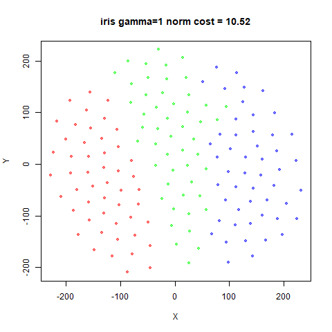
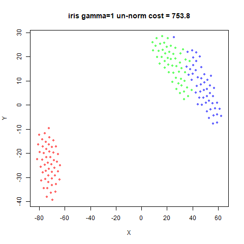
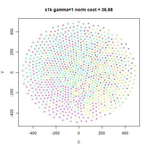
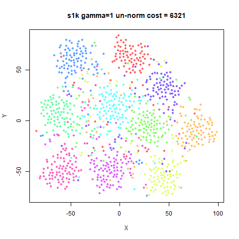
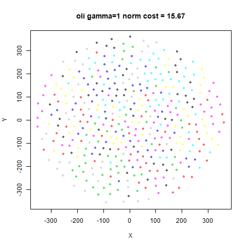
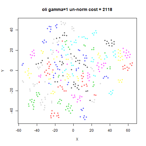
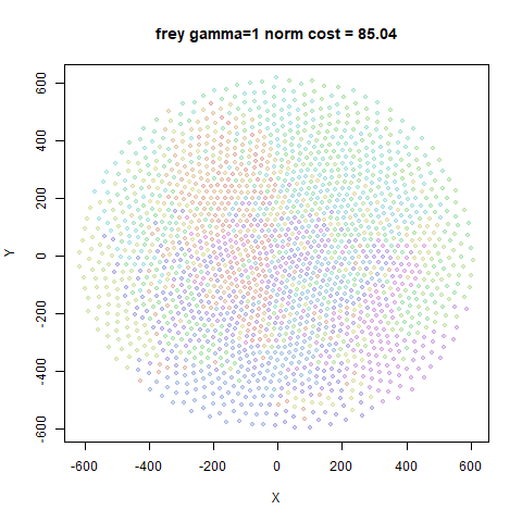
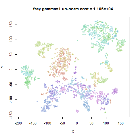
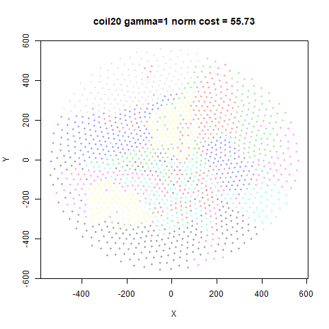
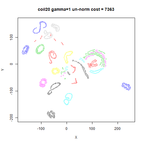
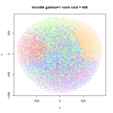
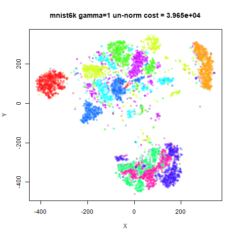
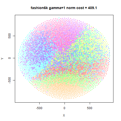
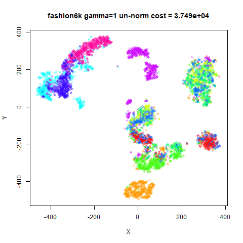
The top row shows the effect of setting gamma = 1 with normalized (left, “norm” in the caption) or un-normalized (right, “un-norm”) LargeVis. These were run for 10000 iterations due to the requirement of a low value of the learning rate. These results are hopefully reasonably converged to give a reasonable depiction of how LargeVis ends up with gamma = 1 using an initialization that works well for t-SNE. But it should be noted that a previous version of this page used 5000 iterations and got results that weren’t very converged. So these could end up changing again.

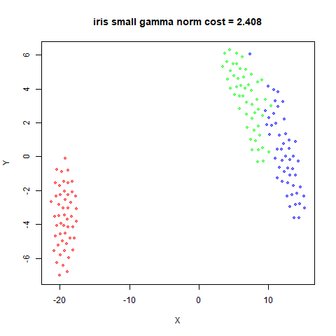
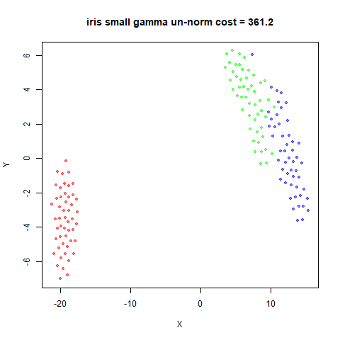
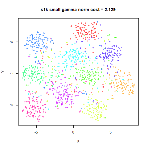
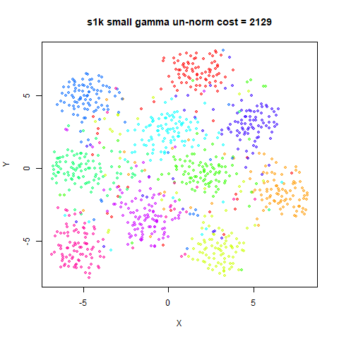
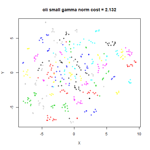
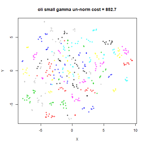
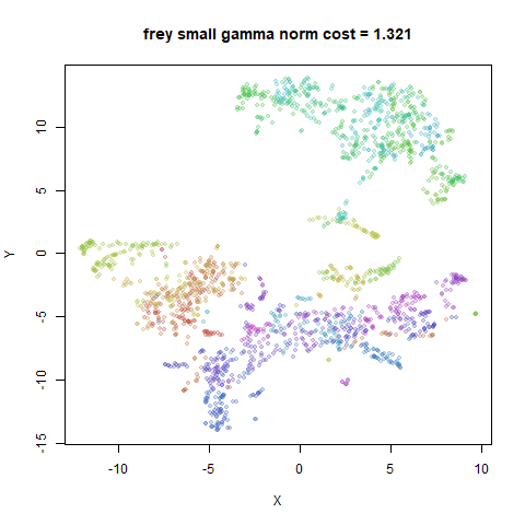
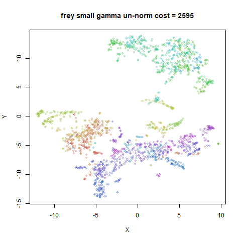
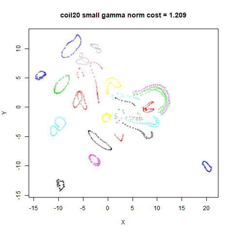
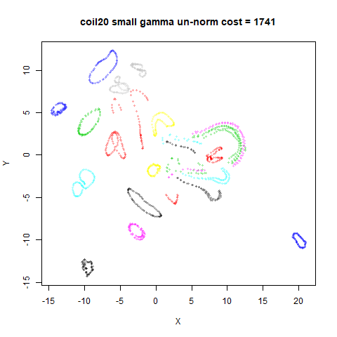
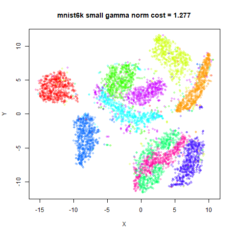
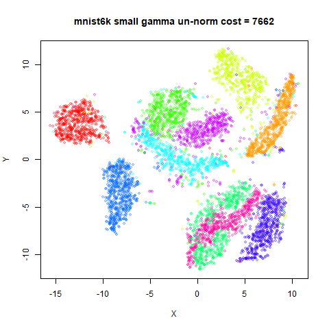
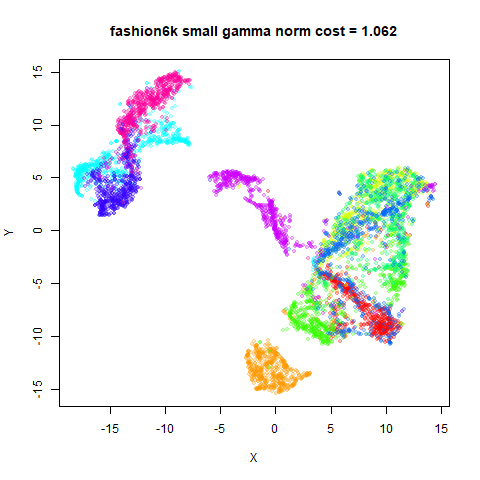
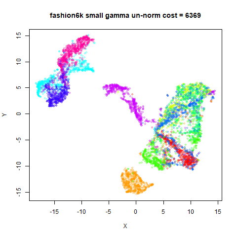
The second row uses a small value for gamma, scaled appropriately for whether we are normalizing or not: 1/N or 1/N^2, respectively. These were able to be run with the typical 1000 iterations.

iris

s1k

oli

frey

coil20

mnist6k

fashion6k

Obviously, gamma = 1 with normalized LargeVis gives disastrously over-repulsed results. Results don’t look terrible with un-normalized LargeVis on the smaller datasets, but things don’t look good with mnist6k or fashion6k. mnist6k in particular is a real mess.

Is this just a case of a bad choice of initialization. Probably not because I’ve used a spectral initialization and random initialization and got the same results. Nor does changing gr_eps affect the results very much, except for the worse if you make it too small (results not shown).

The second row results with a small gamma look better for all the datasets and get there with one tenth of the number of iterations.

Annealed-gamma results

Given the similarity of the LargeVis gradient to t-EE, and given that t-EE results with a larger repulsion improve notably if you start with a small value of its \lambda parameter which entirely analogous to \gamma parameter of LargeVis, we can probably expect to see an improvement by doing the same here.

For these runs, I started with \gamma set to a power of 10 closest to 1/N (using arguments I made on the t-EE page to do with what the initial repulsion in t-SNE is like) for un-normalized LargeVis. For normalized LargeVis, I used the power of 10 closest to 1/N^2. Then each run was repeated with gamma increased by a power of 10 and initializing with the final coordinates from the previous run. This was repeated up to and including gamma = 1. For un-normalized LargeVis, this involved 3-5 round of optimization, and 4-8 for normalized LargeVis.

The total number of iterations allowed was 10000, the same as for the results with gamma = 1 in the previous section. The 10000 iterations were equally divided among each gamma. If a run finished early, the unused iterations were shared amongst the remaining runs equally. Because runs with higher values of gamma tend to take longer to optimize, this allowed these “spare” iterations to be put to good use.

Choosing a good learning rate that works for all values of gamma is tricky. For un-normalized LargeVis, eta = 0.1 worked well. For normalized LargeVis, the best value I found was 10/N.

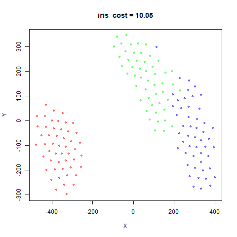
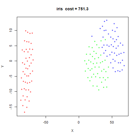
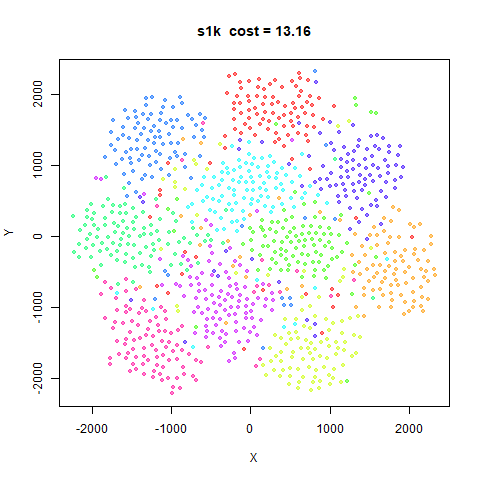
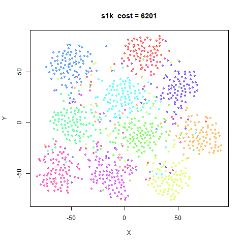
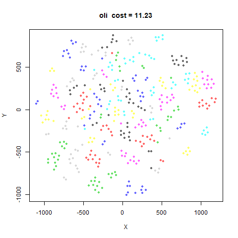
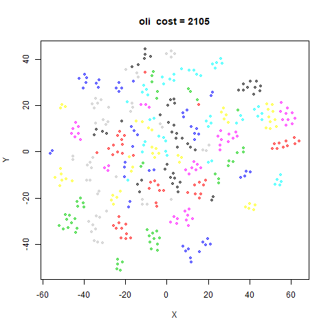
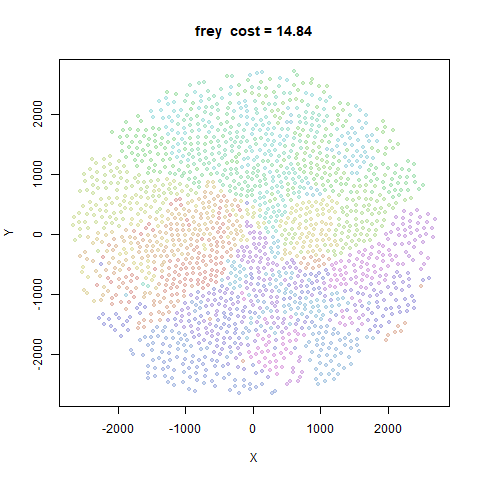
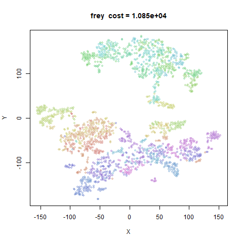
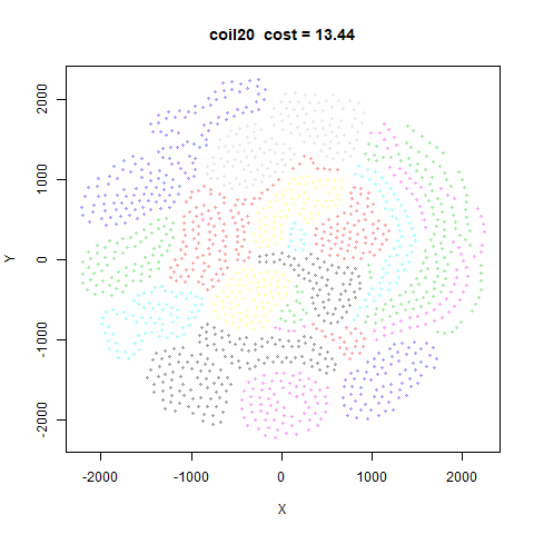
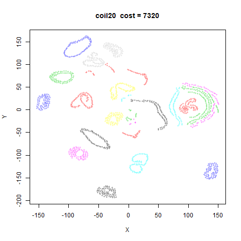
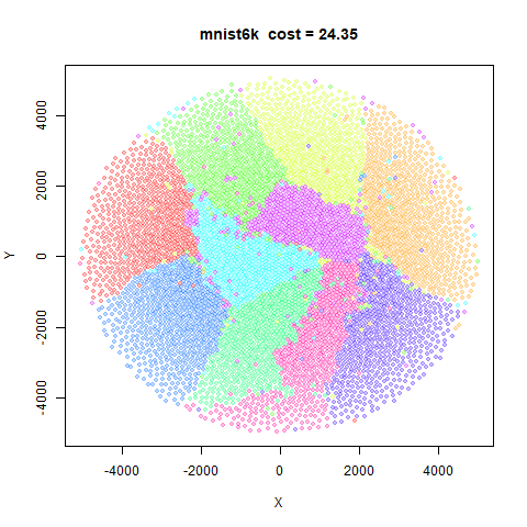
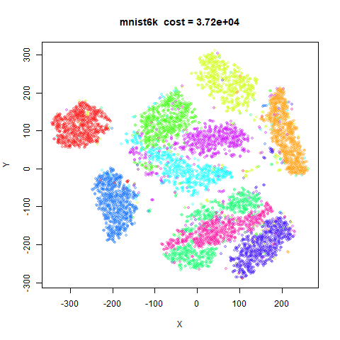
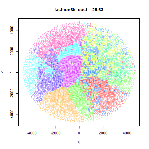
For the results below, I forgot to indicate on the image title whether they were for normalized or un-normalized. Sorry. The normalized LargeVis results are on the left and the un-normalized on the right (but I will repeat this in the section titles)

iris (left: normalized, right: un-normalized)

s1k (left: normalized, right: un-normalized)

oli (left: normalized, right: un-normalized)

frey (left: normalized, right: un-normalized)

coil20 (left: normalized, right: un-normalized)

mnist6k (left: normalized, right: un-normalized)

fashion6k (left: normalized, right: un-normalized)

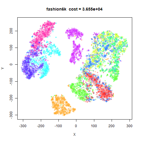The un-normalized LargeVis results are obviously massive improvements. The normalized LargeVis results are less impressive, but better than what came before.

The un-normalized LargeVis results generally converged at all stages, so I am fairly confident those are representative. The normalized LargeVis results are still not fully converged even with 10,000 iterations.

That issue is exacerbated for normalized LargeVis because it starts at a lower value of gamma compared to the un-normalized results, but still ends at gamma = 1, stepping through single powers of ten. Restarting the optimization loses any useful information about the curvature that might have built up which wastes some of the iterations, and also a large chunk of the optimization at each gamma seems to involve the initial expansion of the clusters until they form what look a lot like Voronoi polyhedra, before the clusters shrink and begin to move away. Because it takes a few more values of gamma to get to the target with normalized LargeVis, there are fewer iterations left over for the larger values of gamma to use.

I repeated the coil20 results with the same annealed gamma approach, but allowing up to 100,000 iterations. Results are indeed improved:

COIL-20 embedding using normalized LargeVis with annealed gamma and up to 100,000 iterations.

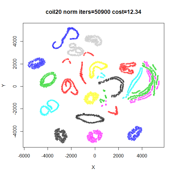
There is still less white space between the clusters compared to the un-normalized results. While it’s obvious the normalized results need further optimizing, I can’t bring myself to spend any more time on that at the moment, so this can stand as evidence of the extra difficult of working with normalized LargeVis (at least with larger values of gamma). Most of the results below will therefore use the un-normalized version.

Early Exaggeration

The annealed-\gamma results tell us that we can probably use whatever value of \gamma we want if we are prepared to get there by starting at a small value and increasing every few iterations. Starting with a reduced repulsion is equivalent to a increased attraction, which is what early exaggeration does. As this is already part of the smallvis interface, maybe this is worth trying.

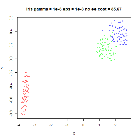
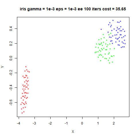
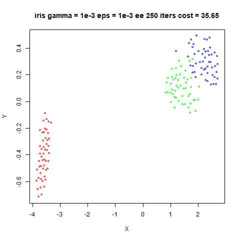
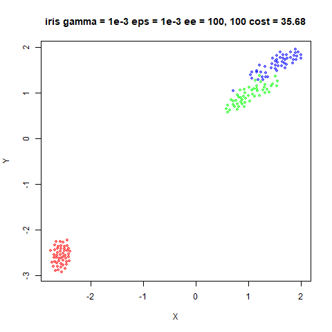
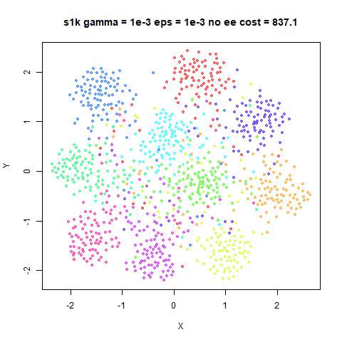
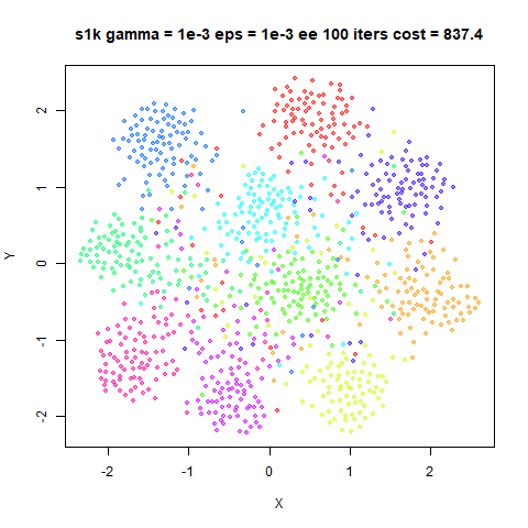
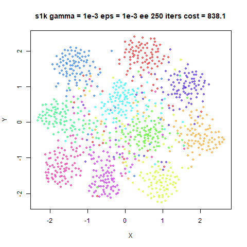
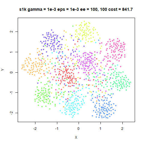
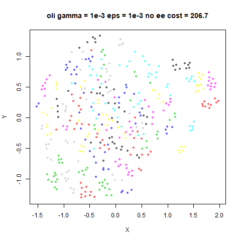
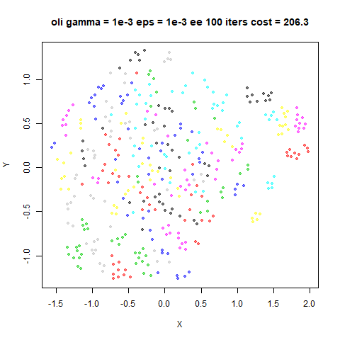
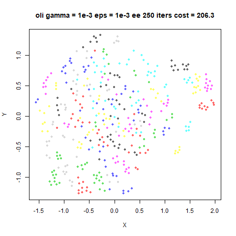
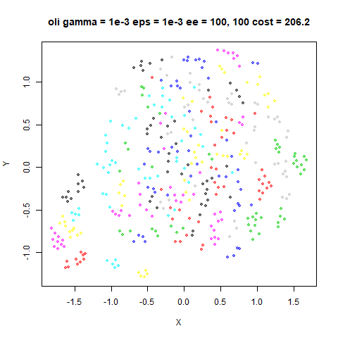
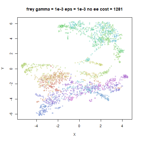
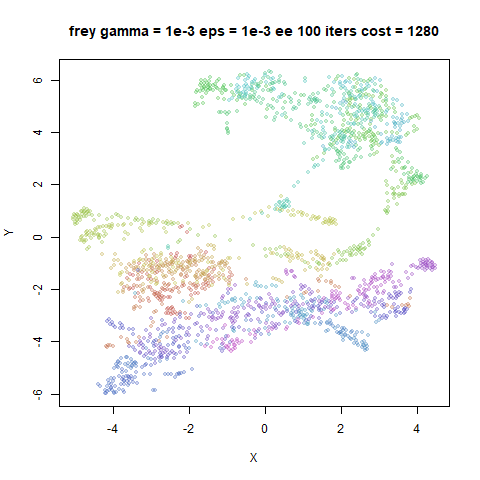
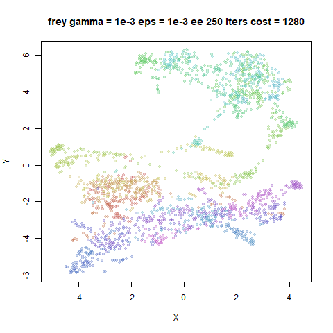
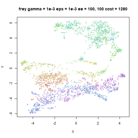
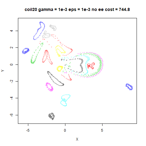
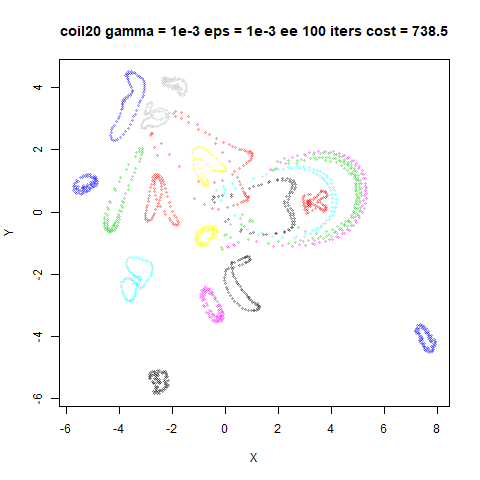
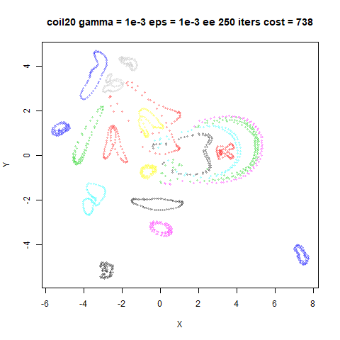
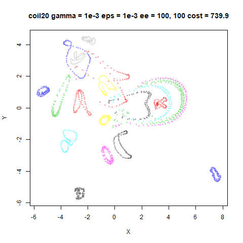
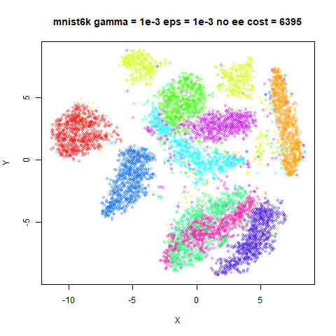
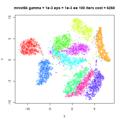
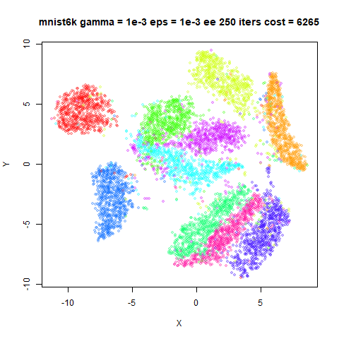
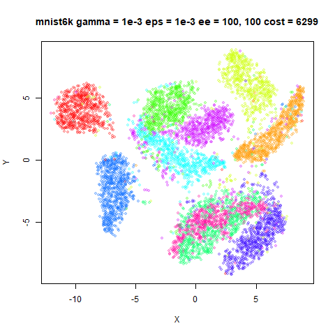
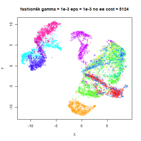
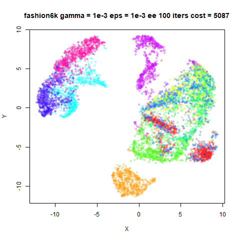
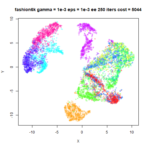
Below are some experiments using gamma = 1e-3, gr_eps = 1e-3. The top left image is what you get without any early exaggeration. Top right is with exaggeration_factor = 10, stop_lying_iter = 100, turning off exaggeration fairly early, and then bottom left is with stop_lying_iter = 250, the more typical exaggeration time used in BH t-SNE. The exaggeration_factor = 10, is the equivalent of starting with gamma set to an order of magnitude lower than we end with. This is more aggressive than the typical t-SNE exaggeration factor of 4. The bottom right image sees if there is an advantage from an even stronger exaggeration_factor = 100.

A typical setting is:

iris_lvee <- smallvis(
  iris,
  method = list("largevis", gamma = 1e-3, gr_eps = 1e-3, normalize = FALSE),
  Y_init = "spca",
  eta = 0.15,
  perplexity = 40,
  g2tol = 1e-7,
  min_cost = -Inf,
  exaggeration_factor = 10,
  stop_lying_iter = 100
)

iris

s1k

oli

frey

coil20

mnist6k

fashion6k

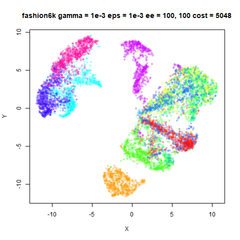For most datasets, early exaggeration doesn’t have much effect, which is perhaps not too surprising as small datasets have more space to arrange themselves. For mnist6k and fashion6k there is a more obvious improvement to the final cost, and in mnist6k, the visual output looks a bit better. Increasing the exaggeration_factor = 100 doesn’t seem to help. This means that the range of effective gamma you can use even with early exaggeration is still quite small. For example, you won’t get good results with gamma = 1 this way (results are identical to not using early exaggeration). Increasing the exaggeration_factor further will lead to issues with the learning rate being too large in the initial exaggeration phase, as discussed in Clustering with t-SNE, provably.

Normalized Results vs t-SNE

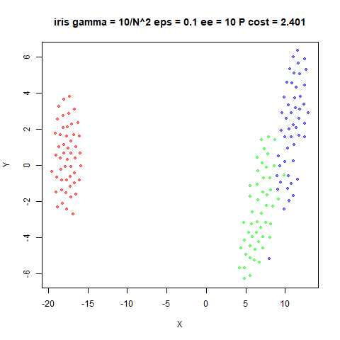
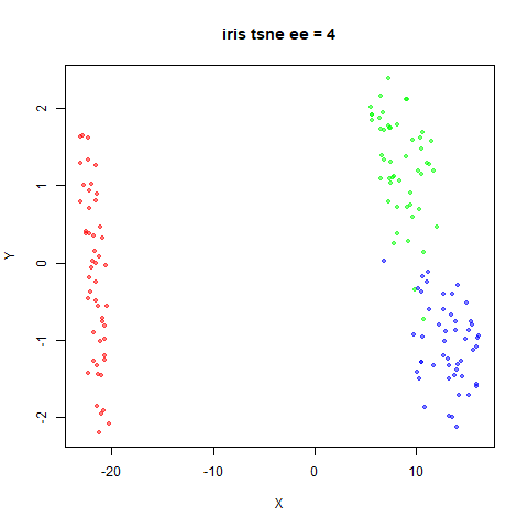
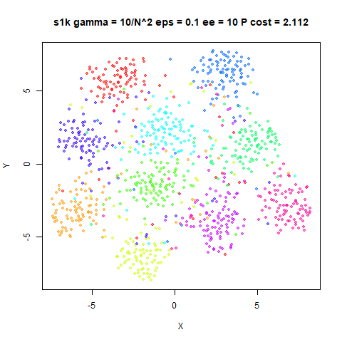
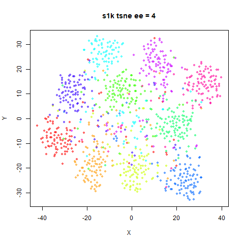
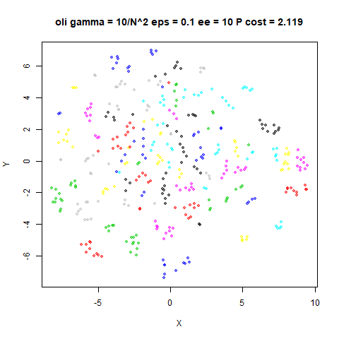
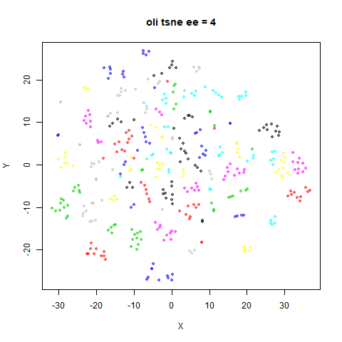
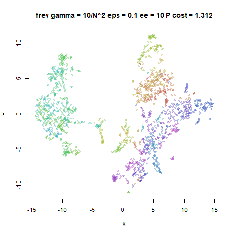
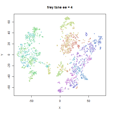
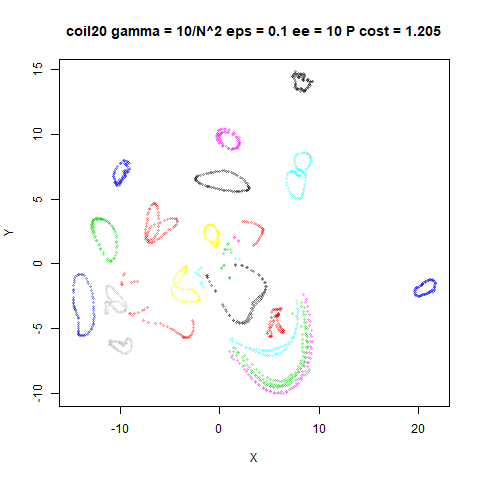
I’ve used un-normalized LargeVis for most of the results above, but to demonstrate that the normalized version of LargeVis, here are some results with the following settings:

iris_lv <- smallvis(
  iris,
  method = list(
    "largevis",
    normalize = TRUE,
    gamma = 10 / nrow(iris)^2,
    gr_eps = 0.1
  ),
  eta = nrow(iris) / 100,
  perplexity = 40,
  g2tol = 1e-7,
  min_cost = -Inf,
  exaggeration_factor = 10,
  Y_init = "spca"
)

This uses a data-dependent \gamma = 10 / N^2 and learning rate of \eta = N / 100. With the exaggeration_factor = 10, this means that the repulsion weight in the gradient will be 1 / N (remember that the repulsion weight is \gamma N in the normalized version of LargeVis) during early exaggeration, which is approximately the initial t-SNE repulsion weight. After early exaggeration the repulsion is reduced by a factor of 10, but remains well below the repulsion weight of around 0.05-0.3 that t-SNE achieves with these datasets and settings. So I anticipate that the LargeVis results will be comparable to, but more compressed than, the t-SNE results.

iris

s1k

oli

frey

coil20

mnist6k

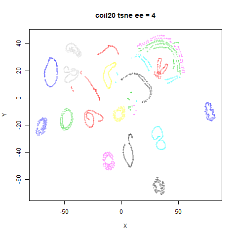
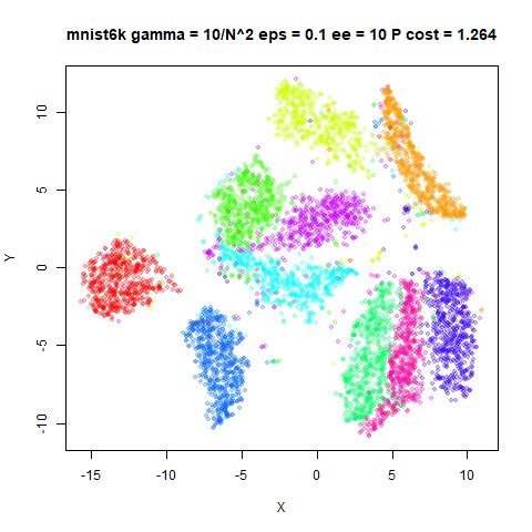
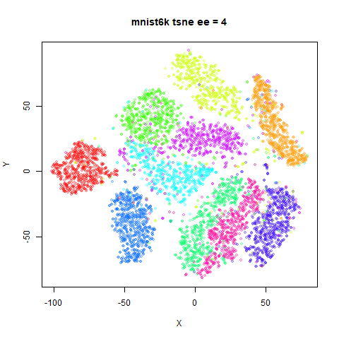
fashion6k

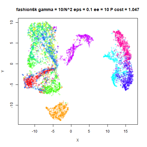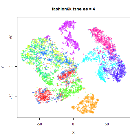This is more or less what I expected. Looking at the range of the axes, the t-SNE results are more expanded but the relative location of the clusters are quite comparable visually (with the exception of iris where the opposite seems true). You can see that for mnist6k and fashion6k, the clusters are more compressed, so it’s probable that the degree of repulsions is size-dependent.

Comparison with SGD results

Finally, let’s compare the results in smallvis to the lvish function in uwot, which should give results fairly close to the “true” LargeVis results. I’m not aiming to reproduce the lvish results in smallvis

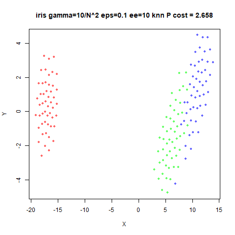
In order to make things more similar, for both smallvis and lvish we will use a knn kernel, where for a given perplexity \mathrm{PP}, the nearest \mathrm{PP} neighbors of point i get an input affinity of 1/\mathrm{PP} and 0 everywhere else. The resulting matrix is symmetrized as usual to get the final v_{ij} values.

For smallvis, the only difference between the previous set of results is adding inp_kernel = "knn" to the method list. For lvish, the settings were:

iris_lvish <- lvish(
  iris,
  n_epochs = 1000,
  kernel = "knn",
  nn_method = "FNN",
  perplexity = 40,
  init = "spca"
)

The choice of n_epochs = 1000 was fairly arbitrary, except it’s double what the default UMAP choice is for small datasets, so hopefully the coordinates are reasonably well converged. Note that lvish is a stochastic method, so exact results are dependent on the random number seed.

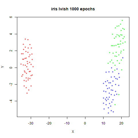
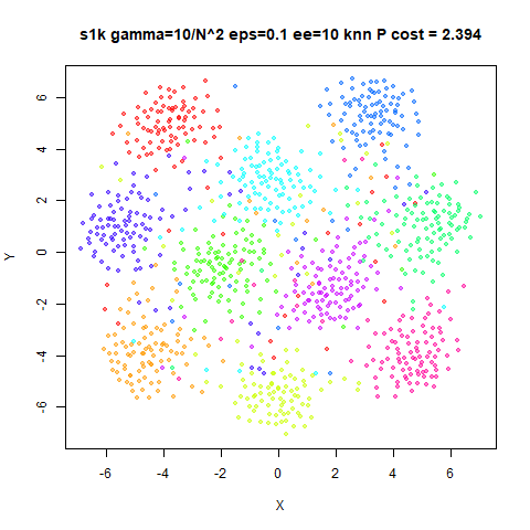
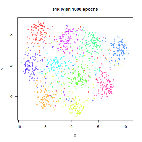
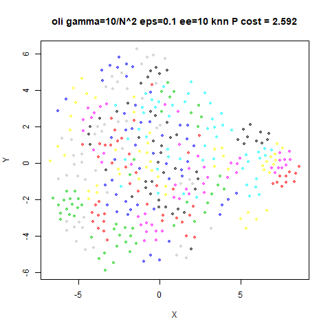
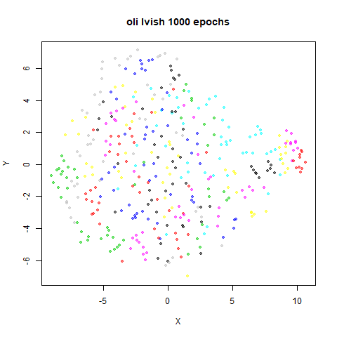
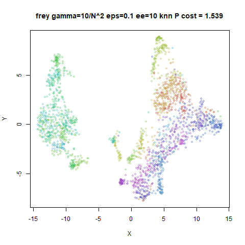
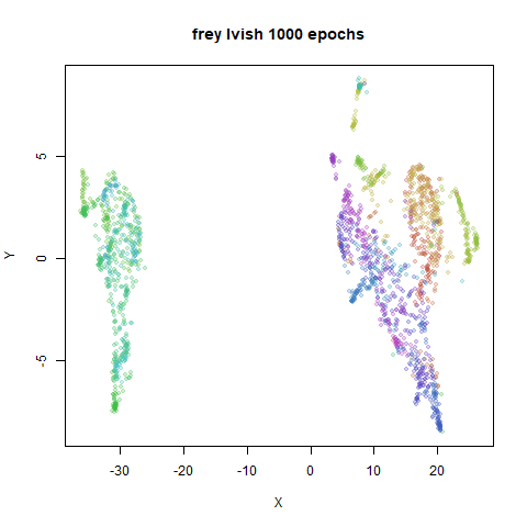
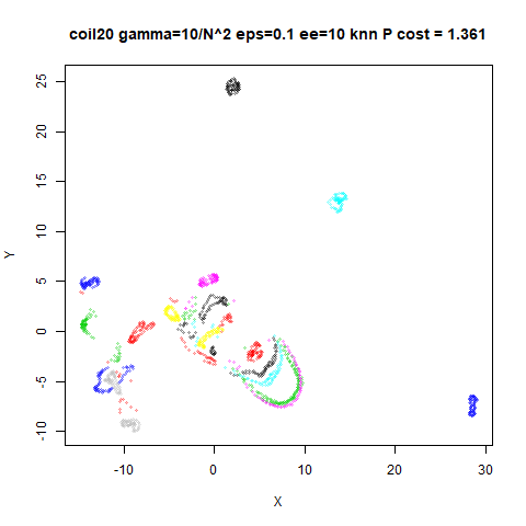
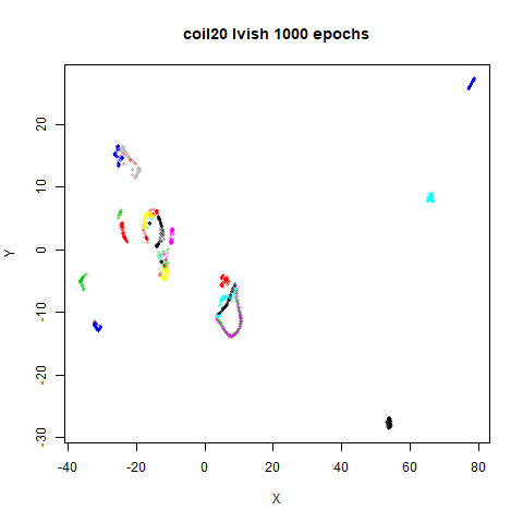
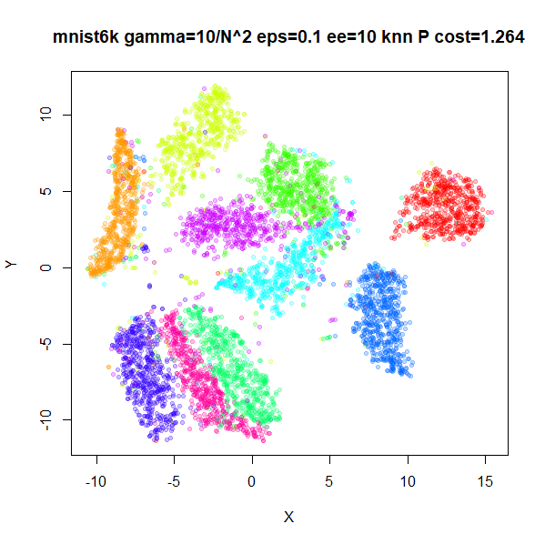
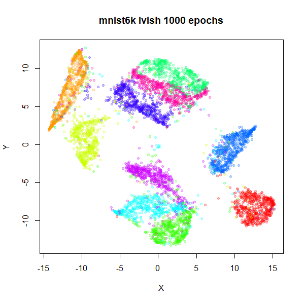
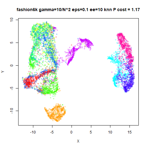
The left-hand result is the smallvis result, the right-hand result is due to lvish.

iris

s1k

oli

frey

coil20

mnist6k

fashion6k

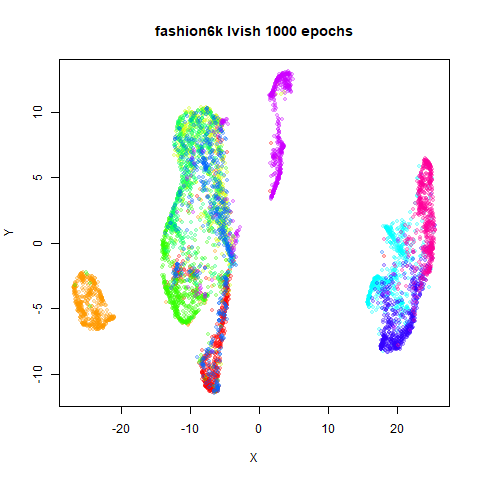Results are most certainly not identical, but they’re not completely different from each other. The chosen value of gamma could perhaps be tweaked to make some visualizations line up better, for example oli seems to be over-expanded in smallvis.

Some differences may be irreconcilable: e.g. for frey, the separation between the green cluster and the rest of the data is always much more pronounced with lvish across multiple random seeds, different choices of n_epochs and learning_rate. For that dataset, even when using smallvis to optimize the output of lvish, I was unable to find a value of gamma which didn’t result in a large amount of re-arrangement of the coordinates. For coil20 there seems to be more expansion with the SGD results and the three clusters (black, cyan and blue) on the right hand side of the plots are pushed further, similarly to the situation with frey.

mnist6k and fashion6k also show a slightly different relative arrangement of clusters. This may be a limitation of the SGD implementation in terms of representing the LargeVis cost function as implemented in smallvis, but this is a mystery I will leave for another time. If it turns out to be due to a bug in uwot, I will regenerate these results.

However, we see similar overall ranges of coordinates (based on looking at the axis labels), so this is good enough evidence for me to confirm that the LargeVis repulsion is substantially down-weighted compared to t-SNE.

Conclusions

LargeVis is not designed to be a practical visualization method outside of its stochastic gradient descent implementation, so the fact that it’s not as easy to use in smallvis compared to t-SNE isn’t very surprising.

Some general observations are:

• Despite sharing a lot of concepts, an un-normalized method like LargeVis is hard to optimize using the techniques that work with t-SNE.
• The problem is both with the optimization method (hyper-parameters including learning rate) and initialization.
• For initialization, I’ve tried increasing the standard deviation of the initial coordiantes (whether using PCA, spectral methods or random) to increase the initial inter-point distance and avoid large gradients, but I was unable to find a useful setting.
• The balance of repulsions versus attractions in the t-SNE family of methods is critical.
• Methods which don’t start the optimization with attractions hugely up-weighted will have a hard time producing useful results.
• t-SNE automatically increases the repulsion as the optimization proceeds, which is why it can produce output with more expanded clusters successfully.
• Early exaggeration helps t-SNE with this. It’s less useful for methods like UMAP or LargeVis because the repulsions don’t get dynamically re-weighted.
• As presented in the LargeVis paper, it’s easy to be misled by the \gamma value in the cost function. Its value > 1 in the stochastic gradient descent optimization, suggests it is up-weighting repulsions relative to the attractive forces.
• Once you recast the SGD settings in terms of the exact gradient, it’s actually strongly down-weighting the repulsions.
• This is still true even when the SGD \gamma = 1, which is effectively what UMAP does.
• This implies that with UMAP’s default settings, its cost function actually contains an implicit \gamma \ll 1.
• In t-SNE, exaggeration is the same as decreasing the repulsive interactions, which is equivalent to introducing \gamma < 1 into the repulsive part of the t-SNE gradient (ignoring a constant scaling of the gradient which can be absorbed into the learning rate). This is why t-SNE with late exaggeration looks like UMAP and LargeVis.
• Therefore t-SNE with exaggeration permanently turned on should give you a close equivalent to (the stochastic gradient descent implementations of) LargeVis or even UMAP visualizations, subject to which implementation provides you with the scalability and features you need.

Turning LargeVis into UMAP

April 26 2020: Dmitry Kobak compared the results above to what I reported about UMAP, and given how close LargeVis should be to UMAP (especially in the t-UMAP form), thought that there were some more things that needed explaining, especially around the results when \gamma = 1. It turns out that he was correct. This new section goes into a bit more detail on the specifics of what separates UMAP from LargeVis.

The results above make clear that having an adjustable \gamma value is important to get good visualizations, and that you probably want \gamma < 1. This seems to conflict with UMAP, which has no \gamma in its cost function. It does appear in the Python implementation (as the repulsion_strength parameter), but its purpose is entirely to account for the missing repulsions due to limited sampling of repulsions in stochastic gradient descent (this was confirmed to me in an email from UMAP creator Leland McInnes). So in its exact-gradient form, there should be no \gamma. That means t-UMAP ought to behave similarly to LargeVis with \gamma = 1, which we know to be difficult to get good results with. In the UMAP pages I do note that UMAP and t-UMAP were quite hard to optimize: that would be in line with my findings here that large values of \gamma make optimizing LargeVis difficult. But we can see from the annealed-\gamma results that with \gamma = 1, we get very expanded clusters, which are not like the t-UMAP results on the UMAP page, which are much more compact. Can we account for this?

The big difference between LargeVis and UMAP is in the affinity calculation: LargeVis does the things the t-SNE way (Gaussian perplexity calibration and symmetrization by averaging) and UMAP uses smooth knn distances and fuzzy set union for symmetrization. Using UMAP input affinities in t-SNE doesn’t make a big difference, but the final matrix normalization may play a role there: before that step, apart from some minor perturbation due to symmetrization, the t-SNE input affinities are normalized to sum to 1, while in UMAP they sum to \log_2 k, with k being the number of neighbors, so analogous to the perplexity setting in t-SNE. The theory of UMAP does not call for any normalization of input affinities to probabilities, so unlike LargeVis there is no confusion over whether you normalize or not: you do not.

Although the individual values of v_{ij} are between 0 and 1 in both methods, the difference in normalization means that there is a lot more total affinity in the smooth knn distances methods, which suggests that the attractive interactions are up-weighted relative to the perplexity-based calibration in t-SNE. This would mean that compared to LargeVis, there is an effective \gamma < 1 in UMAP, which would make the optimization a little easier. But is the reduction in repulsion enough to make a noticeable difference? We can test this in un-normalized LargeVis with different input kernels: inp_kernel = "gauss" for the usual t-SNE perplexity calibration, and inp_kernel = "skd" for the smooth knn distances. For completeness, we’ll also look at inp_kernel = "knn", where each of the perplexity nearest neighbors get an affinity of 1 / perplexity, which was instructive when compared to skd in t-SNE. We’ll also look at averaging (symm = "av") versus fuzzy set union (symm = "fuzzy"). This made little difference with t-SNE, but perhaps the lack of normalization will reveal larger changes.

The results below will be done at two perplexities: perplexity = 40, which is a typical value used in t-SNE, and perplexity = 15, which is closer to the sort of value used in UMAP. For the input_kernel = "skd", the perplexity parameter is interpreted as the number of nearest neighbors.

Rather than go straight to a fully UMAP-like setting with gamma = 1, we’ll use values of gamma that gave reasonable visualizations based on the previous results: \gamma = 10 / N with an initial exaggeration factor of 10 for 100 iterations. An example for iris with perplexity = 15:

iris_ga15 <- smallvis(
  iris,
  method = list(
    "largevis",
    gamma = 10 / nrow(iris),
    gr_eps = 0.1,
    normalize = FALSE,
    inp_kernel = "gauss",
    symmetrize = "average"
  ),
  eta = 0.01,
  Y_init = "spca",
  perplexity = 15,
  g2tol = 1e-7,
  min_cost = -Inf,
  exaggeration_factor = 10
)

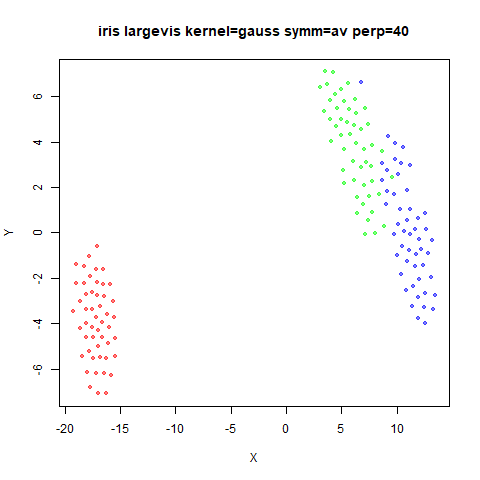
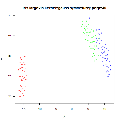
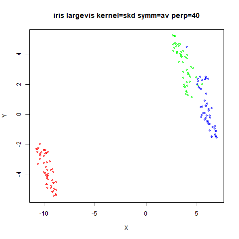
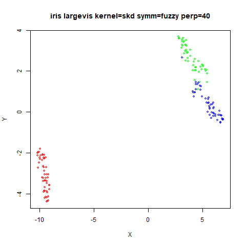
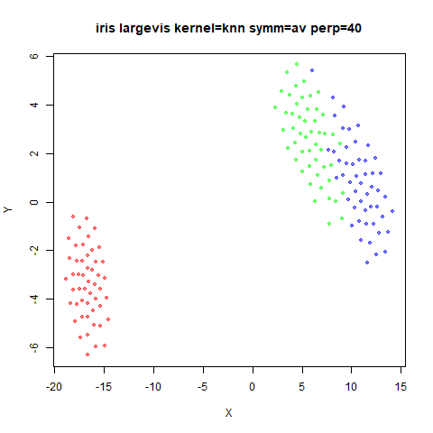
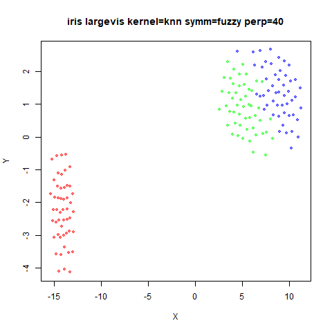
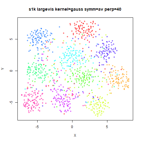
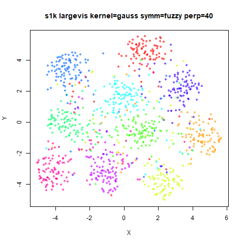
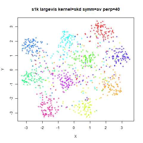
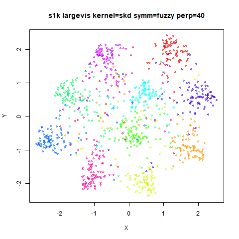
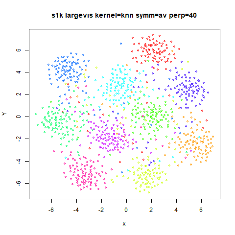
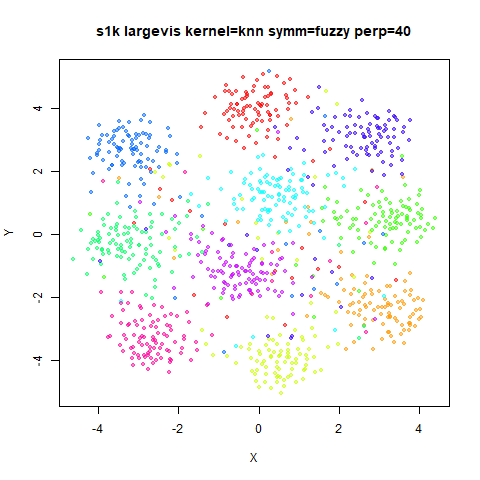
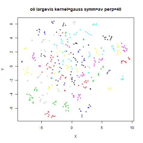
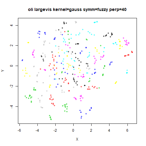
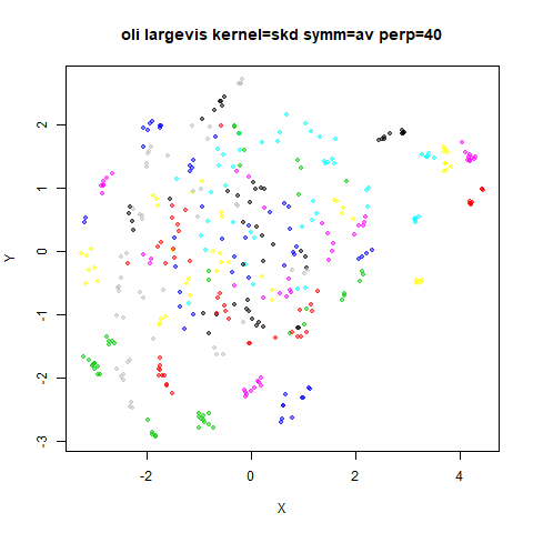
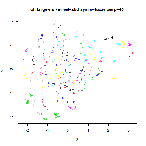
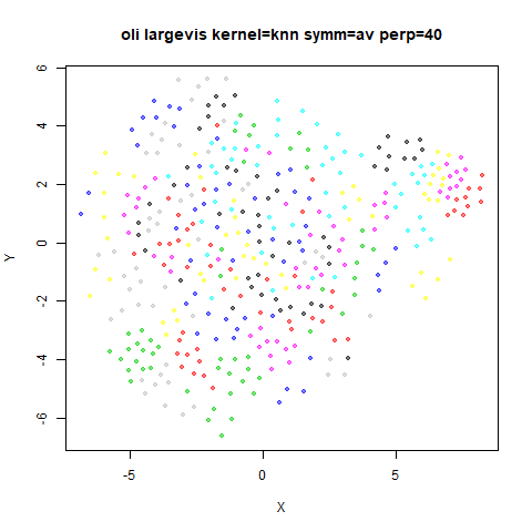
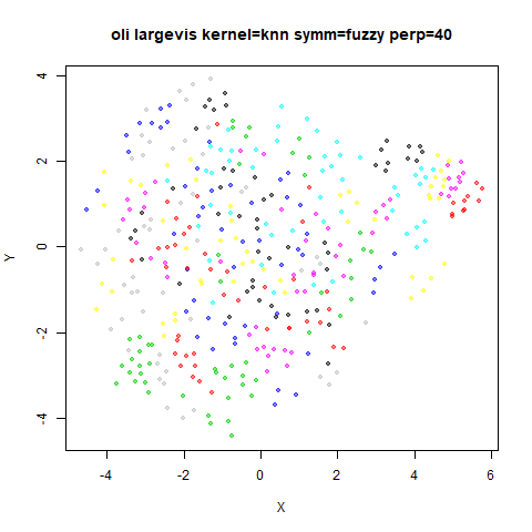
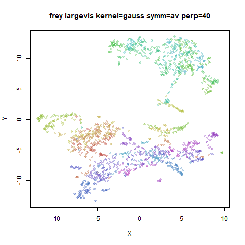
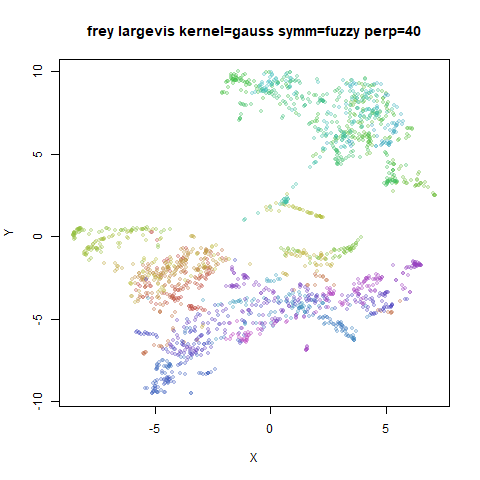
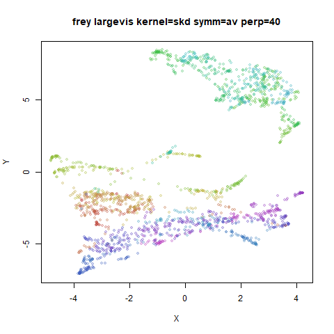
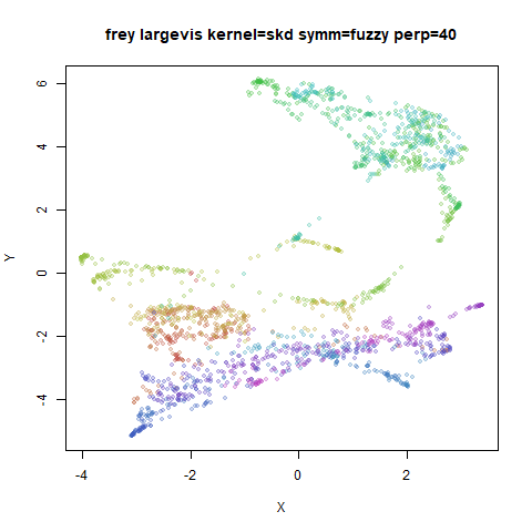
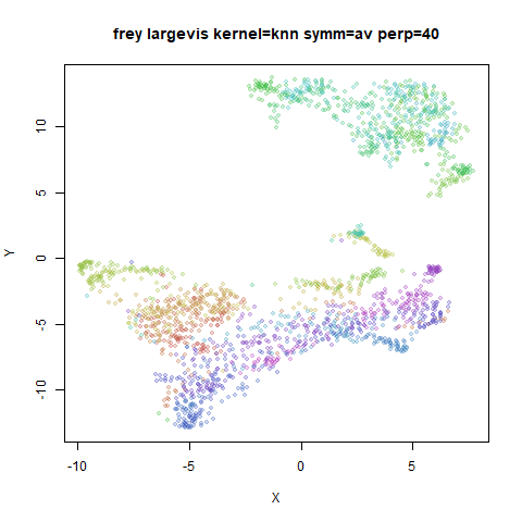
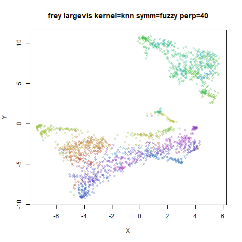
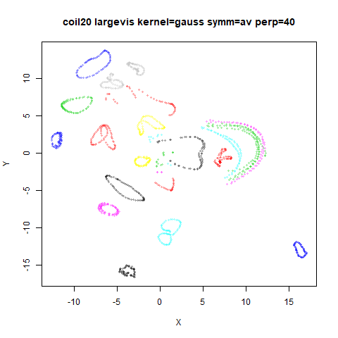
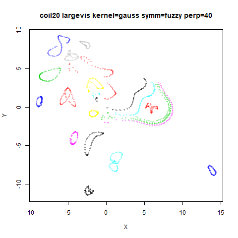
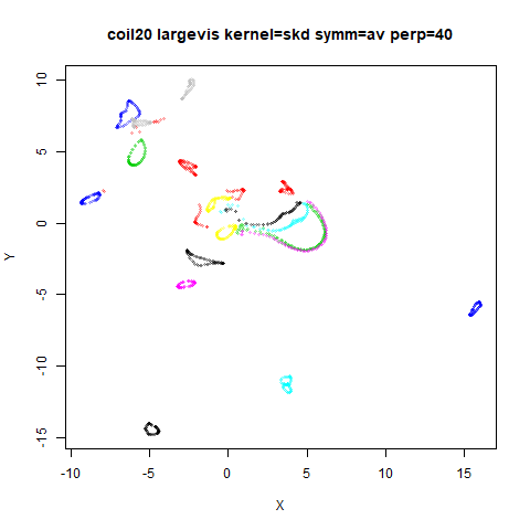
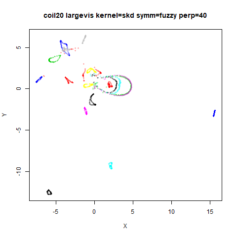
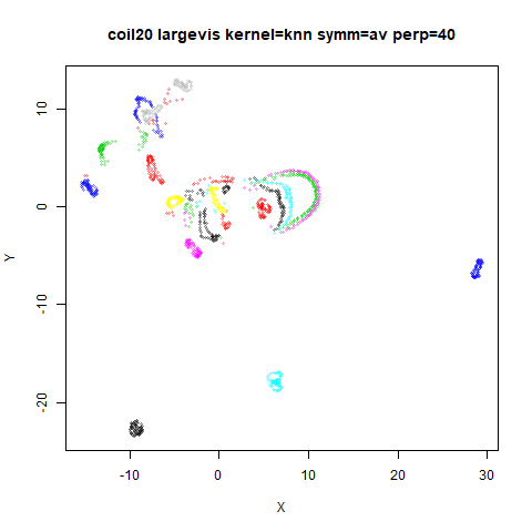
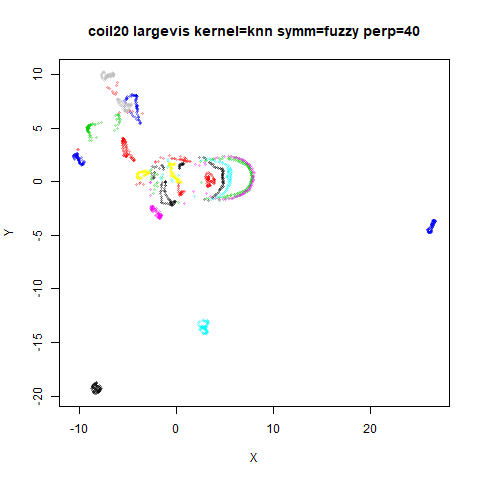
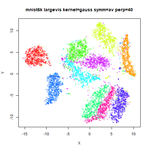
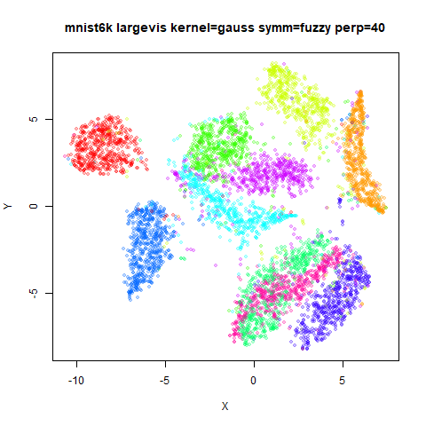
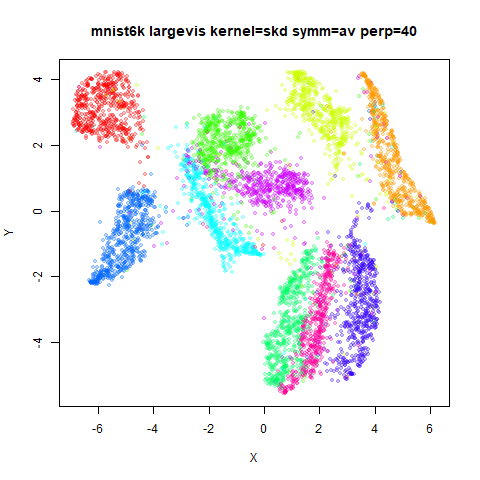
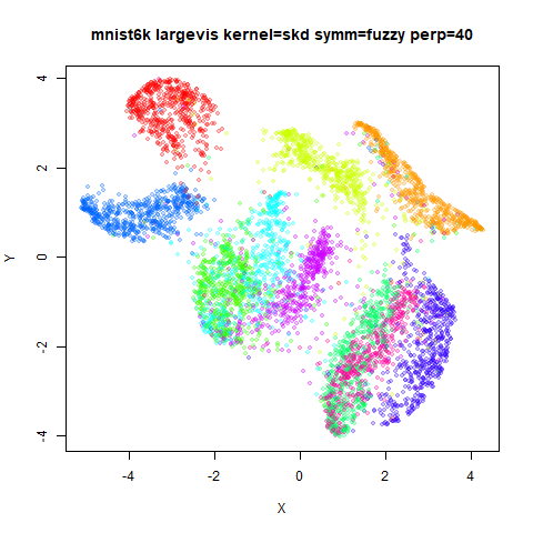
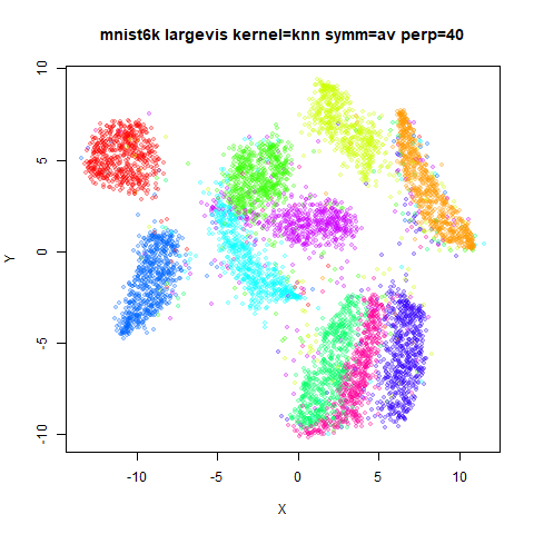
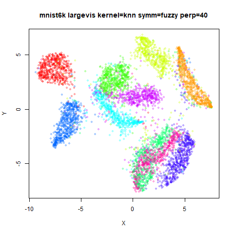
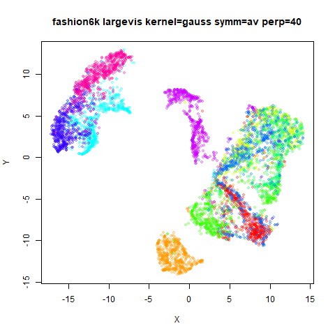
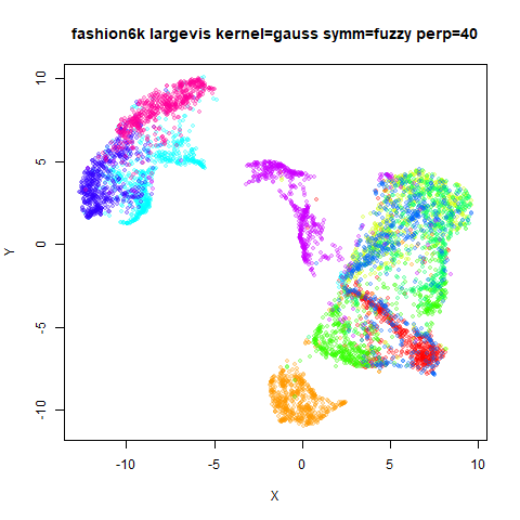
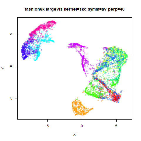
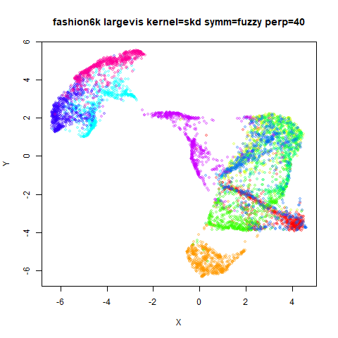
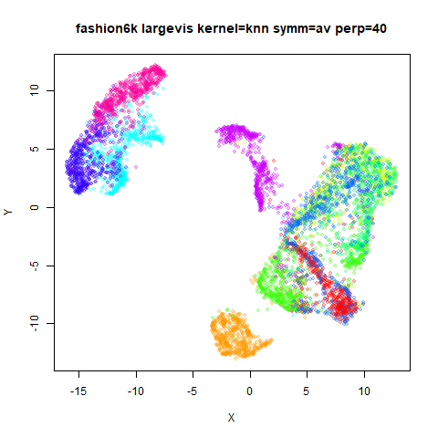
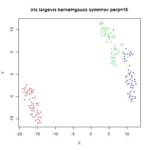
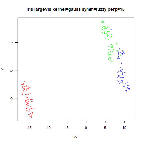
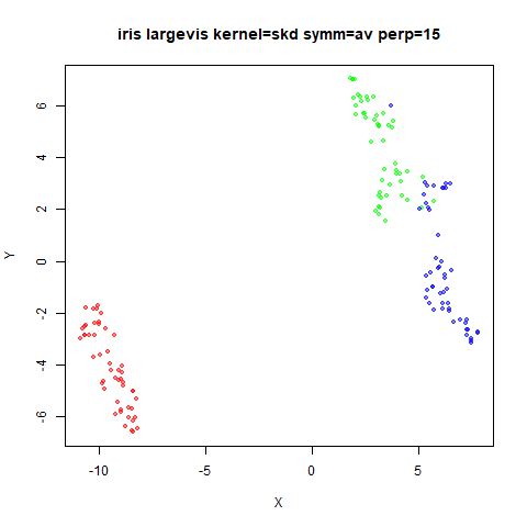
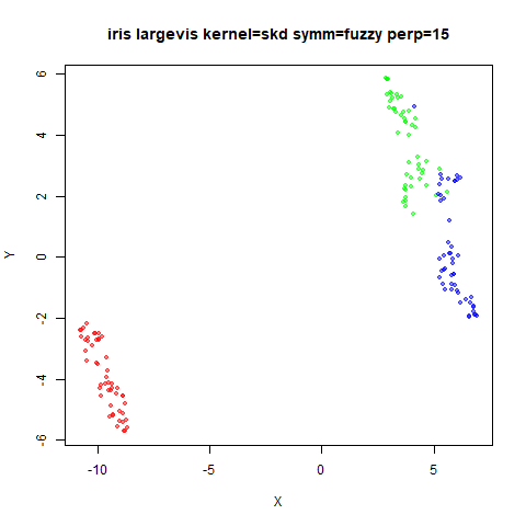
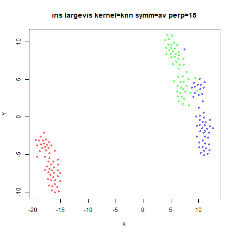
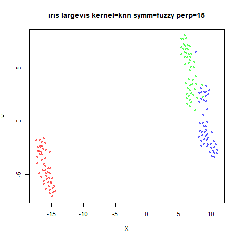
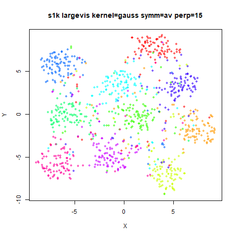
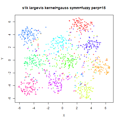
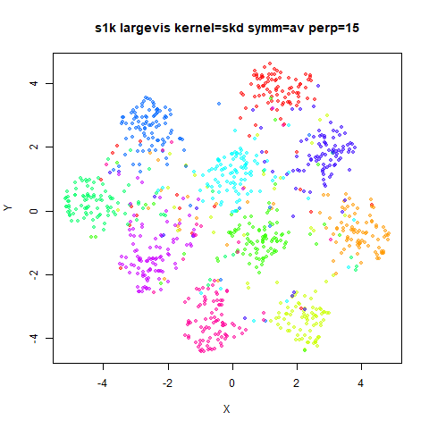
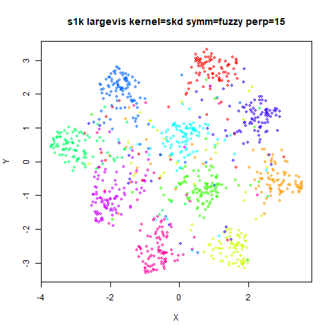
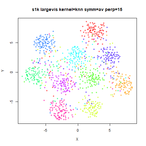
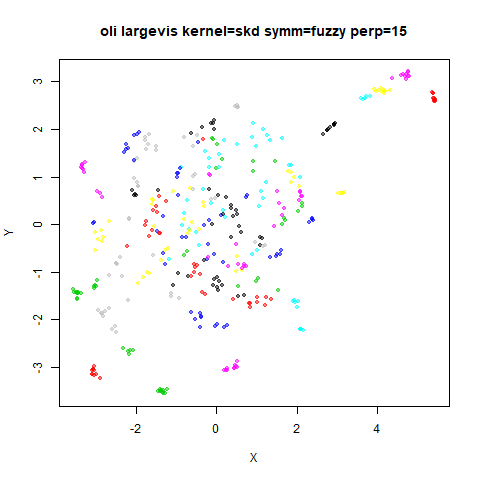
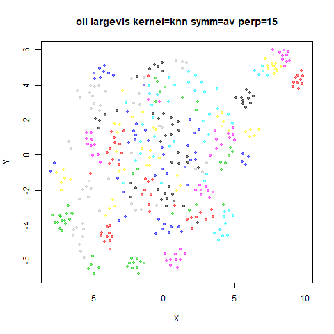
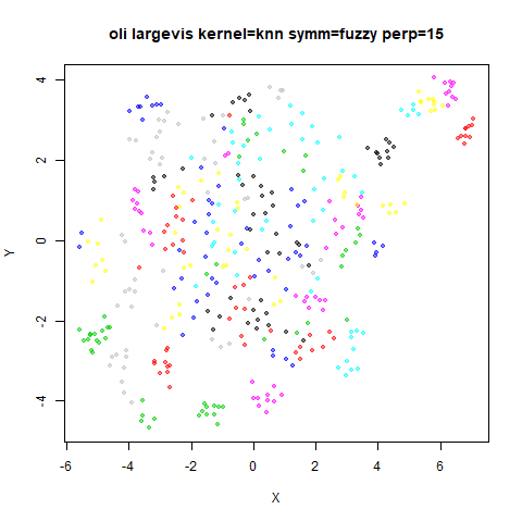
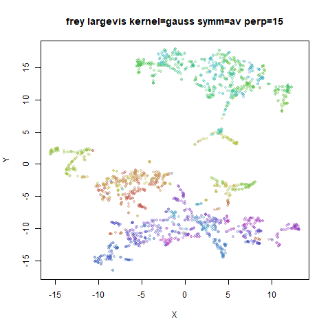
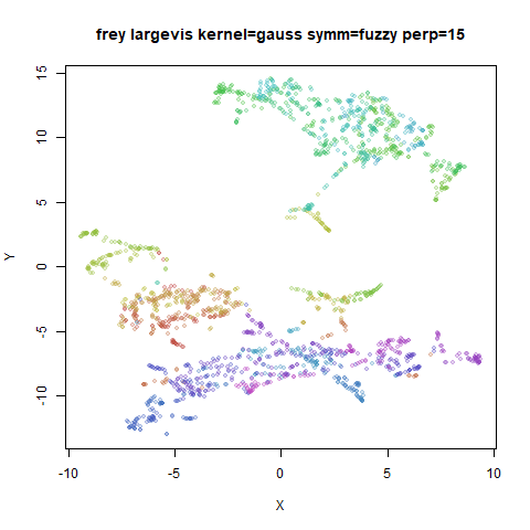
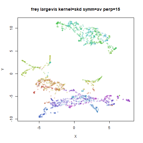
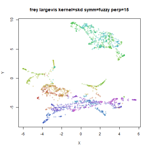
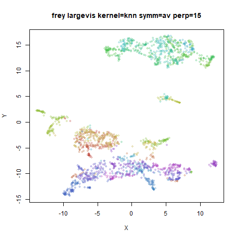
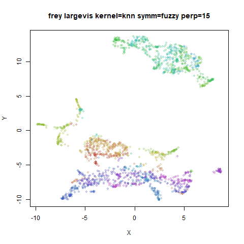
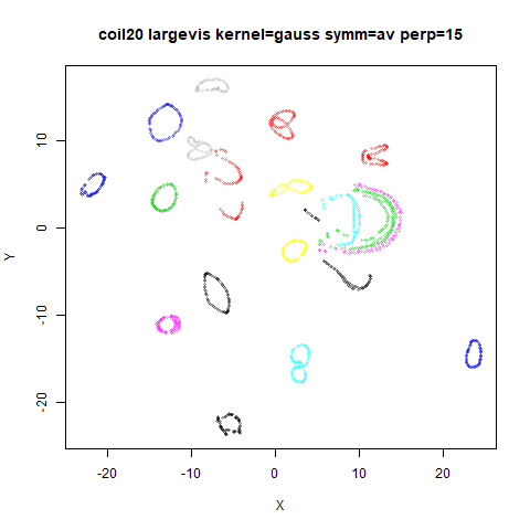
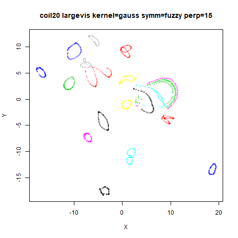
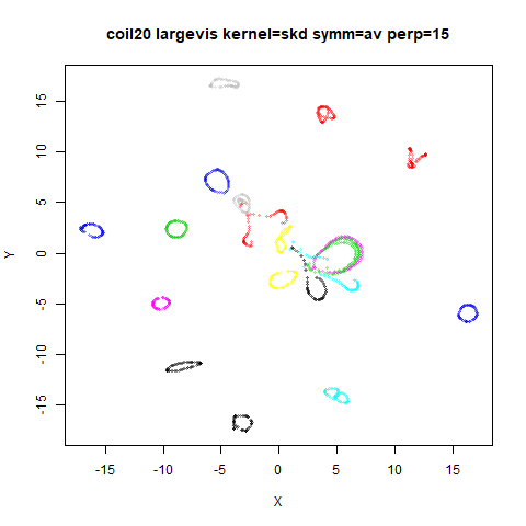
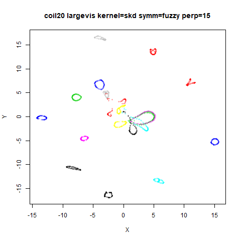
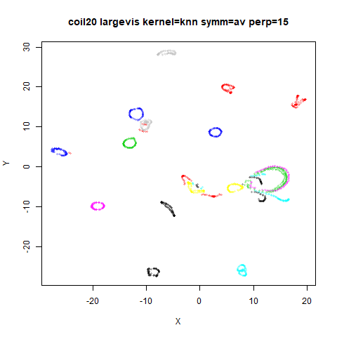
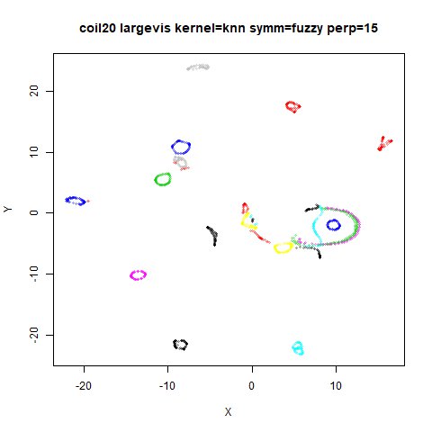
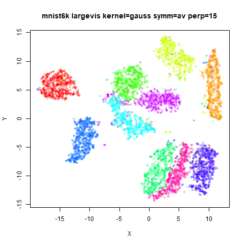
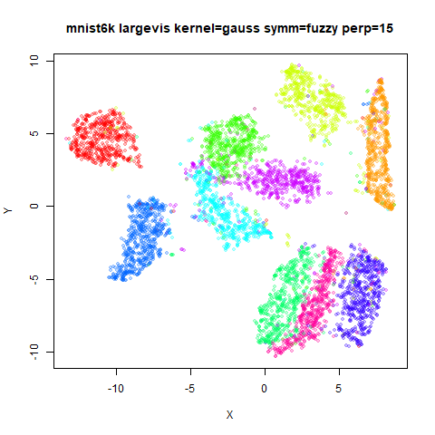
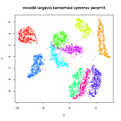
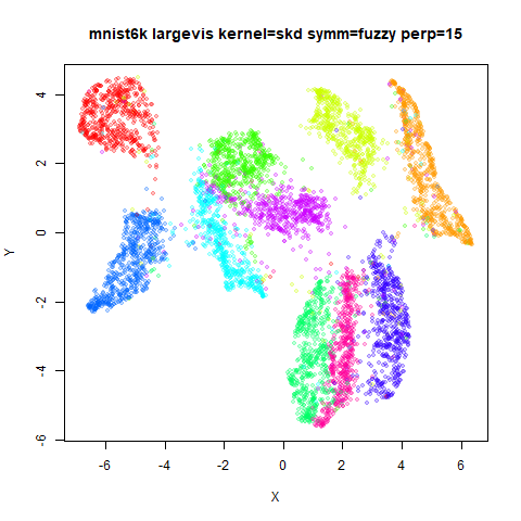
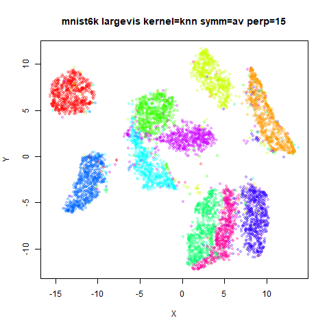
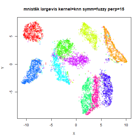
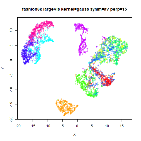
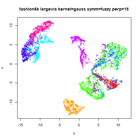
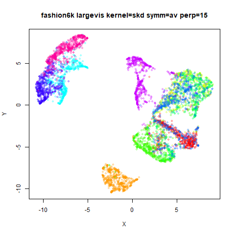
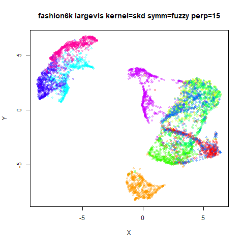
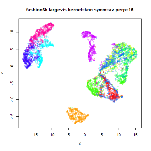
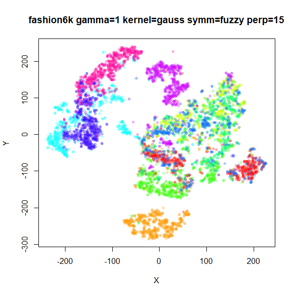
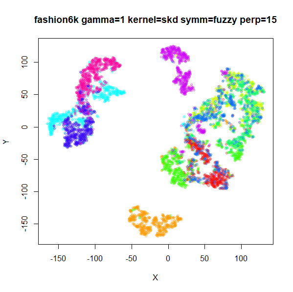
In the results below, the first row uses t-SNE-like perplexity calibration (the LargeVis default). The second row uses smooth knn distances (the UMAP default). The third row uses the k-nearest-neighbors perplexity calibration.

The left hand column uses the averaging symmetrization (LargeVis default), the right hand column uses fuzzy set union (UMAP default).

Results for perplexity = 40 are shown first, then perplexity = 15 in a second section

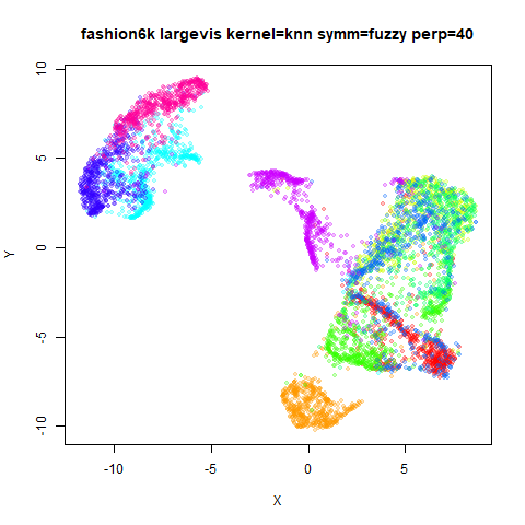
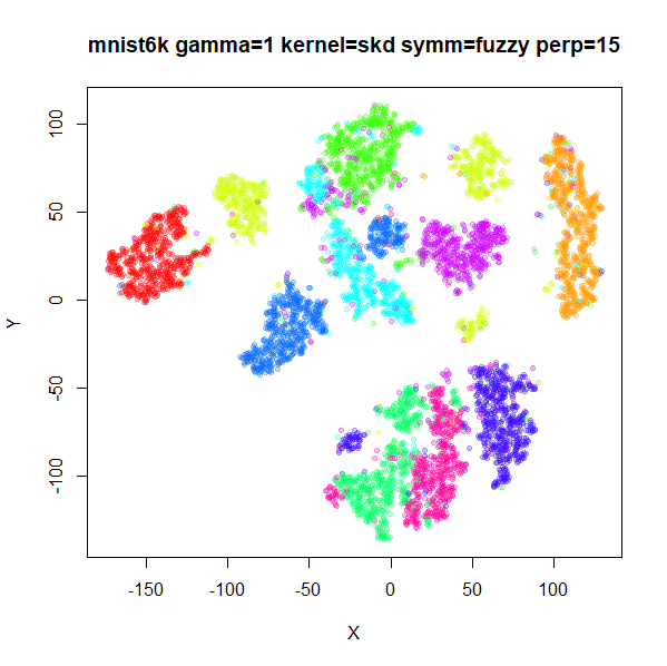
Kernel + Symmetrization Results: Perplexity 40

iris

s1k

oli

frey

coil20

mnist6k

fashion6k

Kernel + Symmetrization Results: Perplexity 15

iris

s1k

oli

frey

coil20

mnist6k

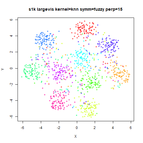
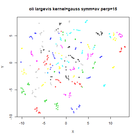
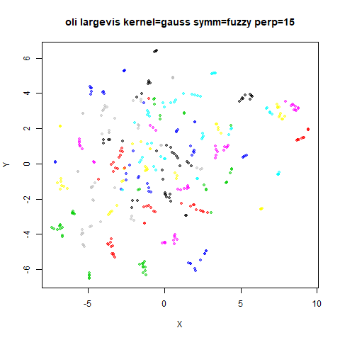
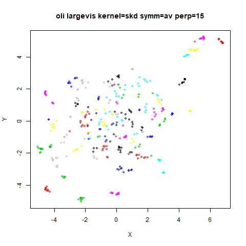
fashion6k

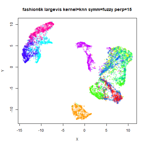For the most part, the effect of symmetrization is almost impossible to detect without peering closely at minor changes. If you look at the knn results for frey with perplexity = 15, you’ll see that there’s a small green/orange cluster of points in the middle of the plot, which is off to the left in all the others. You know things are bad when you’re reduced to noticing that kind of thing. A larger change can be seen with mnist6k with perplexity = 40, where the cerise (thank you name that color) and green cluster in the lower left get entangled with each other when using the fuzzy set union symmetrization. Apart from that, symmetrization does not seem like a big deal with un-normalized affinities.

Also, it doesn’t seem like new behavior in either symmetrization of the input kernel emerges when changing from perplexity = 40 to perplexity = 15, so I will mainly concentrate on the effect of input kernel with perplexity 40, as that lines up with the other LargeVis results on this page.

When looking at input affinities in t-SNE, the smooth knn distances results were somewhere between the Gaussian kernel and the knn kernel. Without matrix normalization, that no longer seems to be the case. There is now a noticeable difference in the amount of repulsion for skd versus gauss (and knn) affinities, with the skd results showing noticeably tighter clusters for iris and oli (also in s1k where the clusters show a more “peaked” or slightly triangular shape), although for coil20 the knn and skd results are quite similar. However what is noticeable for nearly all the plots if you look at the ranges on the axes of the plots is that the skd results take up a much smaller extent. This would seem indicative of a smaller relative repulsion compared to the other kernels.

Initializing t-UMAP and LargeVis from Largevis

So far we’ve seen that the smoothed knn distances input affinities lead to more compressed results than the typical LargeVis Gaussian kernel for a given value of \gamma. However we were using quite low values of \gamma suitable for creating decent visualization with the Gaussian kernel. Do these results hold up when \gamma = 1, which is the effective \gamma used in UMAP?

To test this we are going to focus on just mnist6k and fashion6k, which are the largest datasets and the ones which are most obviously badly affected by using \gamma = 1 without very careful initialization. Also, I am going to switch to using perplexity = 15 now, because I’m now interested in reproducing more UMAP-like behavior with LargeVis.

For a given input kernel, we will run an un-normalized LargeVis optimization with gamma = 1. This is going to be difficult to get good results, so we will also use an exaggeration_factor = 10. Also, we’re going to set the learning rate fairly low, to eta = 0.001, because I’ve noticed that early on in the optimization, there are quite large gradients that can lead to initial distortions (e.g. one or two outlier points that have been displaced a long distance relative to the rest of the data). The visualizations do recover, but as the local minimum they will end up could be quite far from the initial trajectory, which might complicate looking at the final results. To compensate for the lowered the learning rate, we’ll use max_iter = 10000, i.e. ten times long as usual.

We will carry out two runs for each dataset, with input_kernel = "skd" and input_kernel = "gauss" (we won’t look at input_kernel = "knn" so we have less results to sift through, but also because this current set of experiments take so long to complete). My expectations are:

1. Neither results will look that great.
2. The input_kernel = "gauss" results will look worse than the input_kernel = "skd" results.

Then we will use the final coordinates from the LargeVis run to initialize two new optimizations. The two methods are:

• t-UMAP. With the skd kernel initialization, t-UMAP and LargeVis should be very, very similar. So as long as the LargeVis optimization was far enough long to provide a good initialization, I expect the t-UMAP results to not differ very much from the starting point. On the other hand, the gauss initialization should be a worse initialization for t-UMAP and I would expect to see a larger change.
• LargeVis again with the same input kernel parameter as in the first LargeVis run. Apart from restarting the adaptive optimization parameters this is like running a 20,000 iteration optimization. This is more of a control run to ensure that 10,000 iterations was sufficient to get a good initialization for t-UMAP and to track any further changes to the layout that would have occurred anyway. Mainly this is to account for the scenario where LargeVis with the Gaussian kernel gives a bad output, and running t-UMAP on it substantially improves it. Do I expect this to happen? No. But if it did, it would leave the question open as to whether LargeVis just needed longer to optimize those coordinates and would have got there as well as t-UMAP did.

These will also be run for 10,000 iterations and the same learning rate.

To summarize, there will be two sets of three visualizations each:

1. An initial LargeVis run with inp_kernel = "gauss".
2. A LargeVis run with inp_kernel = "gauss" initialized from LargeVis in step 1.
3. A t-UMAP run initialized from LargeVis in step 1.

Then we will repeat all that but with inp_kernel = "skd" in steps 1 and 2. Got it? No? Eh, I did my best.

Here’s an example of the settings we’ll use for the three steps using mnist6k and inp_kernel = "gauss"

mnist6k_lv1 <- smallvis(
  mnist6k,
  eta = 0.001,
  method = list(
    "largevis",
    gr_eps = 0.1,
    normalize = FALSE,
    inp_kernel = "gauss",
    symmetrize = "fuzzy",
    gamma = 1
  ),
  Y_init = "spca",
  perplexity = 15,
  g2tol = 1e-7,
  min_cost = -Inf,
  exaggeration_factor = 10,
  max_iter = 10000,
  epoch = 100,
  tol_wait = 2000
)

mnist6k_lv2 <- smallvis(
  mnist6k,
  eta = 0.001,
  method = list(
    "largevis",
    gr_eps = 0.1,
    normalize = FALSE,
    inp_kernel = "gauss",
    symmetrize = "fuzzy",
    gamma = 1
  ),
  perplexity = 15,
  verbose = TRUE,
  max_iter = 10000,
  epoch = 100,
  Y_init = mnist6k_tu2,
  tol_wait = 2000
)

mnist6k_tu3 <- smallvis(
  mnist6k,
  eta = 0.001,
  method = list("tumap", gr_eps = 0.1),
  perplexity = 15,
  verbose = TRUE,
  max_iter = 10000,
  epoch = 100,
  Y_init = mnist6k_lv1,
  tol_wait = 2000
)

I use the tol_weight = 2000 parameter here, which prevents stopping the optimization before iteration 2000 (after which the final momentum has kicked in for a few hundred iterations). This is to stop the optimizations in steps 2 and 3 from prematurely converging if the adaptive learning rates were taking a while to make progress. Also gr_eps = 0.1 for all methods. I did some preliminary checking to see if this was interfering with accurate gradient values and preventing convergence but it didn’t seem to be an issue.

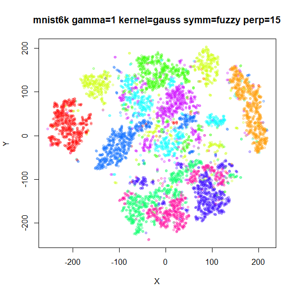
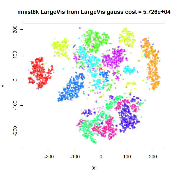
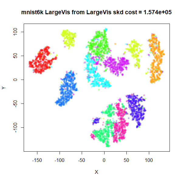
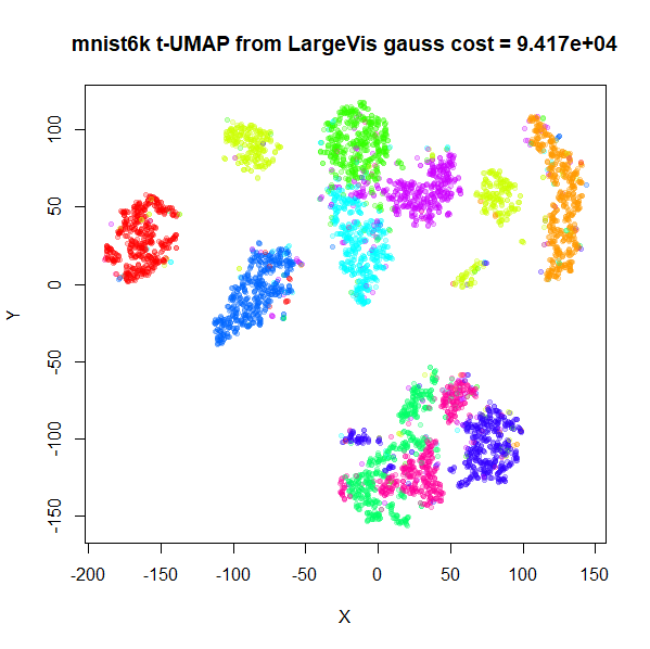
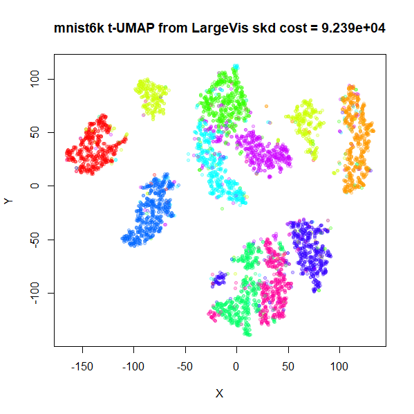
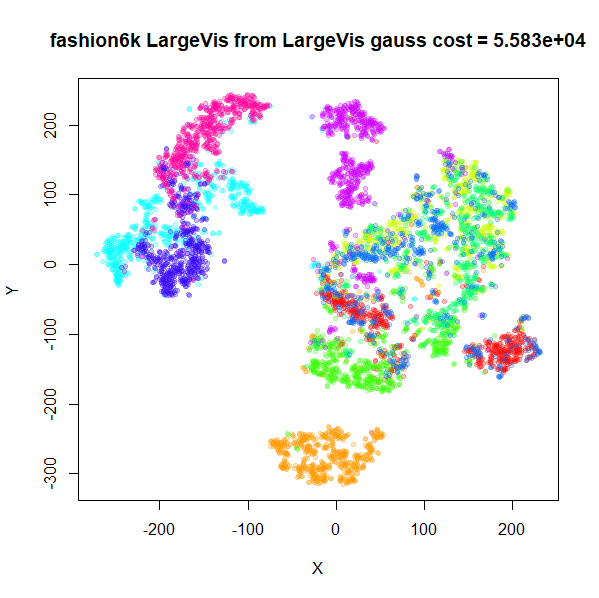
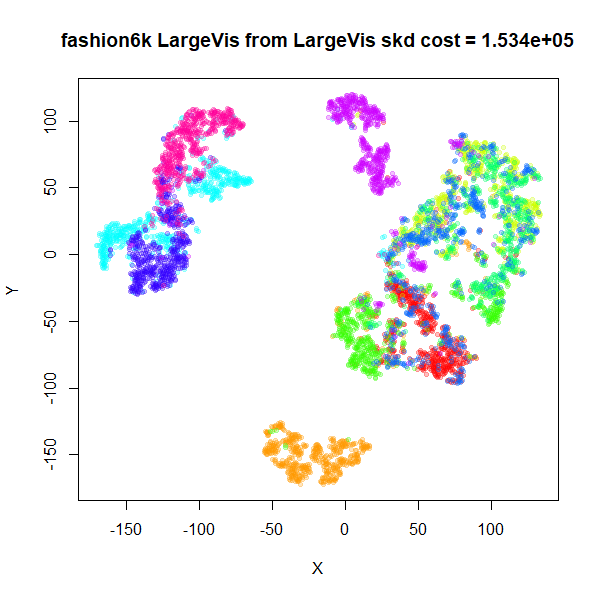
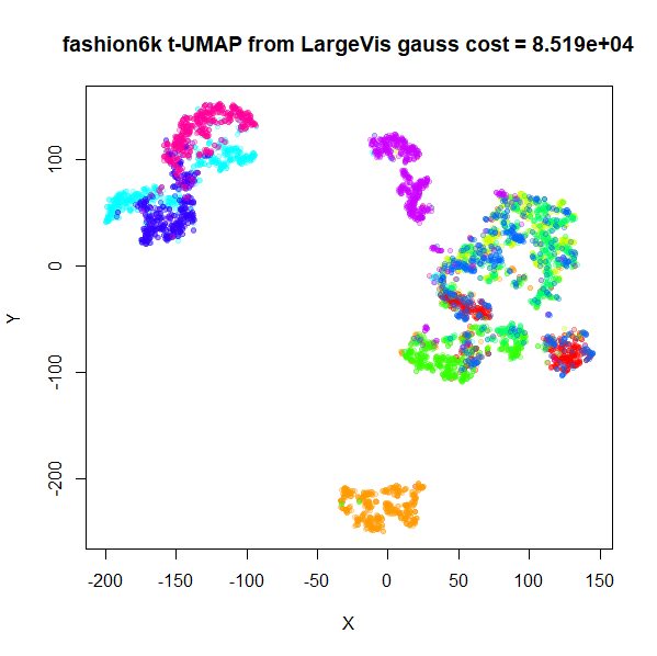
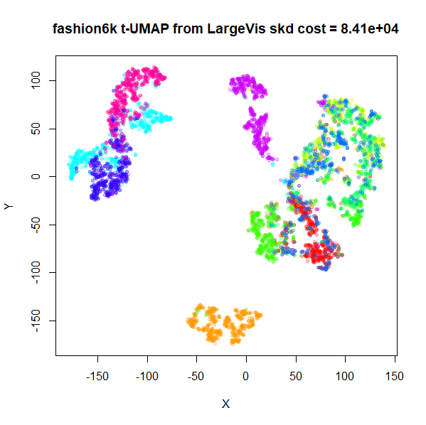
Below the results on the left show the Gaussian kernel and results on the right show the smooth knn distances kernel. Row 1 is the initial LargeVis result, row 2 is the LargeVis result initialized from the first LargeVis result, and row 3 is the t-UMAP result initialized from the first LargeVis result.

mnist6k

fashion6k

mnist6k results are the most instructive to look at, as the Gaussian kernel gives the worst results initially (top left), so any improvement is easier to see. First, note that switching to the smooth knn distances with LargeVis (top right) does help quite a bit, so that behavior seems to hold up even at higher \gamma values. Results are still far from perfect however, with several clusters split.

The middle row is from running LargeVis for another 10,000 iterations, to check if the top results are converged. And there are not major changes. There is certainly some improvement to the inp_kernel = "gauss" results (middle left), but still a long way from what we would like to see. The inp_kernel = "skd" results also improve with some clusters being unsplit. This is important for evaluating the t-UMAP results as that means we can’t attribute these improvements to t-UMAP specifically.

The t-UMAP results are on the bottom row. First, the effect of the smooth knn distances kernel on the gaussian kernel input (bottom left) is very noticeable: results are much cleaner looking than was achieved by just running LargeVis for longer, although the overall arrangement of the visualization is unchanged. As expected, the clusters are smaller, tighter and more well-separated.

On the bottom right we see very little difference from the t-UMAP results compared to the LargeVis results (center right). If you look very closely you’ll see that the fine structure within each cluster seems more pronounced: i.e. the holes inside each cluster are slightly larger. This can be explained by the extra 1 - v_{ij} weighting factor that exists in the repulsions for UMAP compared to LargeVis: The affinity matrix with smooth knn distances is sparse by design so for most pairs of points the repulsion is identical between LargeVis and UMAP. However, for close neighbors in the input space, there is a non-zero v_{ij} so there is an extra down-weighting of repulsions. This pulls the neighbor points closer together, leading to the slightly lower homogeneity inside the clusters. The final cost values in the caption on the bottom row confirm that initializing t-UMAP from input_kernel = "skd" LargeVis results not only leads to more pleasant-looking initializations, but a lower cost.

The fashion6k results confirm the observations above, albeit in less emphatic fashion.

An obvious big difference between the smooth knn distances kernel and the Gaussian kernel is the attractive interactions are stronger by a factor of \log_2 \mathrm{PP} (where \mathrm{PP} is the perplexity), which should be the same as reducing \gamma by the same amount (e.g. setting approximately gamma = 0.25) and then increasing the learning rate accordingly:

mnist6k_lvg <- smallvis(
  mnist6k,
  eta = 0.005,
  method = list(
    "largevis",
    gr_eps = 0.1,
    normalize = FALSE,
    inp_kernel = "gauss",
    symmetrize = "fuzzy",
    gamma = 1 / log2(15)
  ),
  Y_init = "spca",
  perplexity = 15,
  g2tol = 1e-7,
  min_cost = -Inf,
  exaggeration_factor = 10,
  max_iter = 10000,
  epoch = 100,
  tol_wait = 2000
)

MNIST subset embedding with smoothed k-nearest-neighbor input affinities and an annealed gamma schedule.

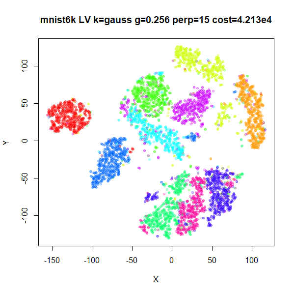
This looks a lot more like the first skd result for (top right image for mnist6k) than the original gauss kernel result (top left), so a difference in effective gamma should be considered when comparing LargeVis to UMAP. However, the difference in the distribution of the affinities (i.e. Gaussian versus the truncated exponential) doesn’t seem to be critical.

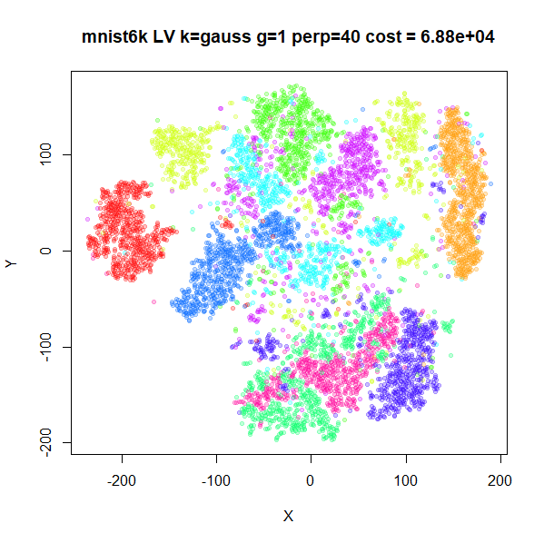
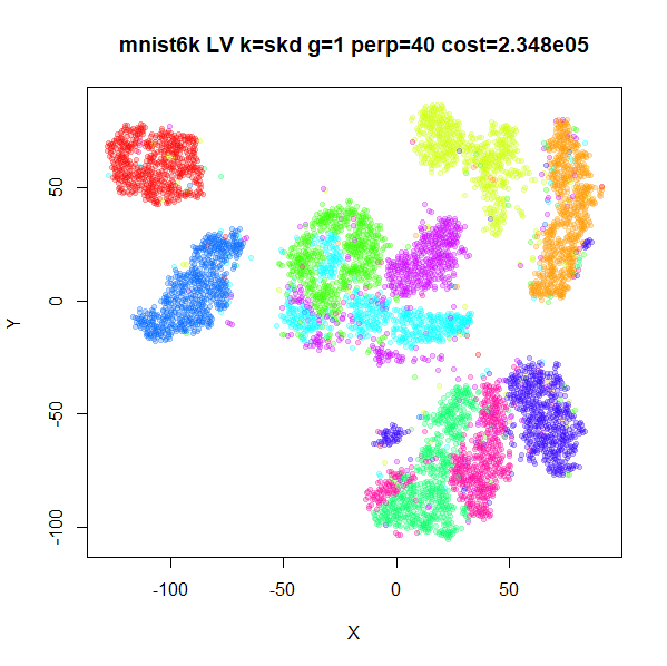
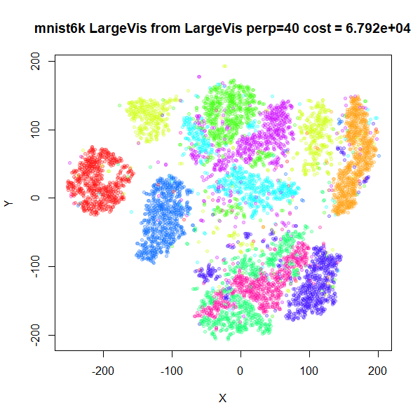
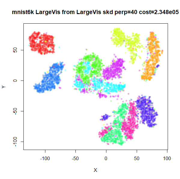
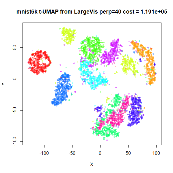
mnist6k perplexity 40

To end this section, here are the mnist6k results with perplexity = 40:

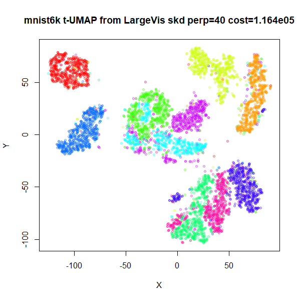These are pretty similar to the perplexity = 15 results in terms of the size and spacing between the clusters, so there doesn’t seem to be a large effect of perplexity on the overall shape of the embedding. The green, cyan and magenta clusters in the middle of the plot are entangled in a different way to the perplexity = 15 results. I looked to see if initializing an extra t-UMAP optimization with perplexity = 15 could un-entangle them, but that is not the case.

Conclusions (Again)

When I was looking at using UMAP input affinities in t-SNE, I concluded that those findings (that nothing made a huge difference) wouldn’t necessarily transfer to un-normalized methods, especially with regard to smooth knn distances. It turns out that this is the case.

1. The use of smooth knn distances in the input affinity means that UMAP has a smaller effective repulsion than LargeVis with its Gaussian input kernel and gamma = 1. With the default parameters of using 15 nearest neighbors, this is equivalent to approximately gamma = 0.25 in the LargeVis case.
2. t-UMAP results will therefore not resemble un-normalized LargeVis with gamma = 1 (they should be less spread out) and won’t be quite so hard to optimize.
3. It’s still quite hard to optimize though.
4. There are lots of things that make optimizing UMAP and LargeVis difficult in their exact gradient form: setting the correct gr_eps value to avoid division by zero, balancing repulsive and attractive interactions, using a good initialization, learning rate. Lots of these considerations are problems for any method, including t-SNE, but they are particularly thorny for un-normalized methods.
5. UMAP is actually at a disadvantage over LargeVis when it comes to the exact gradient optimization: we don’t have a gamma value to modify. An alternative is to use t-SNE-style early exaggeration and multiply the input affinities by a constant factor, but because the UMAP cost function has a \log[(1 - v_{ij}) / (1 - w_{ij})] in it so you have to be careful how that is carried out, e.g. update for the purpose of gradient calculation, but not for the cost function calculation and be careful with any early stopping criteria that use the cost function.
6. However you do it, as we have seen, there are limits to how effective a one-off boost to the repulsion is with un-normalized methods once \gamma becomes large: either the boost is too small to give the desired effect, or the learning rate has to be made very small to accomodate the very different scales of the gradient before and after the exaggeration. A different adaptive learning rate method to the t-SNE Delta-Bar-Delta method (or changes to the parameters) may be needed, which is a lot of work.

Acknowledgement

Dmitry Kobak has been asking me to look at how the smallvis version LargeVis behaves for ages, as well as asking “don’t you think it’s odd that t-SNE with exaggerations looks so much like UMAP?”, so I have him to thank for prodding me into looking at this in a bit lot more detail.