Metric MDS

Can an optimizer recover a recognizable map of Europe from a table of road distances? We will use that problem to explore three parts of the mize callback interface: capturing fixed data in a closure, checking an analytic gradient, and sharing intermediate calculations between the objective and gradient.

datasets::eurodist contains road distances in kilometres among 21 European cities. We will fit a two-dimensional configuration whose Euclidean distances approximate those values. Roads need not follow straight lines, and the cities lie on the curved surface of the Earth, so an exact two-dimensional Euclidean fit should not be expected.

This example minimizes raw stress directly. stats::cmdscale() follows the classical-scaling route and uses a different criterion.

Stress and its gradient

Let \(R = (r_{ij})\) be the target distances and let \(D = (d_{ij})\) be the Euclidean distances among candidate coordinates \(Y\). We minimize raw stress:

\[ C(Y) = \sum_{i < j} (r_{ij} - d_{ij})^2. \]

The condition \(i < j\) counts each unordered pair once. The matrix implementation below instead sums both symmetric triangles, so it multiplies that sum by one half. With \(n\) objects, the corresponding distance RMSE is \(\sqrt{C / {n \choose 2}}\) and has the same units as the input distances.

For distinct points, the derivative with respect to the coordinates of object \(i\) is

\[ \frac{\partial C}{\partial \mathbf{y}_i} = -2 \sum_{j \ne i} \frac{r_{ij} - d_{ij}}{d_{ij}} (\mathbf{y}_i - \mathbf{y}_j). \]

Implementation note. Euclidean distance is nondifferentiable when two candidate points coincide. distance_epsilon prevents division by zero in the code, although the mathematical derivative remains undefined at an exactly coincident configuration. The gradient check therefore uses a seeded, nondegenerate point.

The callback factory captures the fixed target matrix in a closure. Its prepare() helper performs the shared conversion from a parameter vector to coordinates and pairwise distances. A counter records how often that work is performed.

distance_epsilon <- 1e-10

make_mmds_callbacks <- function(
  distances,
  combined = FALSE,
  epsilon = distance_epsilon
) {
  target <- as.matrix(distances)
  preparation_count <- 0L

  prepare <- function(par) {
    preparation_count <<- preparation_count + 1L
    coordinates <- matrix(par, ncol = 2, byrow = TRUE)
    list(
      coordinates = coordinates,
      distances = as.matrix(stats::dist(coordinates))
    )
  }

  stress <- function(prepared) {
    0.5 * sum((target - prepared$distances)^2)
  }

  gradient <- function(prepared) {
    weights <- (target - prepared$distances) /
      (prepared$distances + epsilon)
    coordinates <- prepared$coordinates
    result <- matrix(
      nrow = nrow(coordinates),
      ncol = ncol(coordinates)
    )

    for (i in seq_len(nrow(coordinates))) {
      differences <- sweep(-coordinates, 2, -coordinates[i, ])
      result[i, ] <- colSums(differences * weights[, i])
    }

    as.vector(t(result)) * -2
  }

  callbacks <- list(
    fn = function(par) stress(prepare(par)),
    gr = function(par) gradient(prepare(par))
  )
  if (combined) {
    callbacks$fg <- function(par) {
      prepared <- prepare(par)
      list(
        fn = stress(prepared),
        gr = gradient(prepared)
      )
    }
  }

  list(
    fg = callbacks,
    preparations = function() preparation_count,
    reset_preparations = function() {
      preparation_count <<- 0L
      invisible(NULL)
    }
  )
}

The separate variant supplies fn and gr. The combined variant also supplies fg, which lets mize request an objective and gradient from one prepared configuration.

target_distances <- datasets::eurodist
set.seed(42)
initial_par <- rnorm(attr(target_distances, "Size") * 2)

separate_callbacks <- make_mmds_callbacks(target_distances)
combined_callbacks <- make_mmds_callbacks(
  target_distances,
  combined = TRUE
)

Validate the gradient

check_mize_gradient() compares the analytic gradient with central finite differences. Because the combined callback is present, it also checks that fg agrees with the separate fn and gr callbacks.

gradient_check <- check_mize_gradient(
  combined_callbacks$fg,
  initial_par
)

gradient_summary <- data.frame(
  max_abs_error = gradient_check$max_abs_error,
  max_rel_error = gradient_check$max_rel_error,
  fg_fn_abs_error = gradient_check$fg_consistency$fn$abs_error,
  fg_gr_max_abs_error =
    gradient_check$fg_consistency$gr$max_abs_error
)
knitr::kable(
  signif(gradient_summary, digits = 4),
  row.names = FALSE,
  col.names = c(
    "Maximum absolute error",
    "Maximum relative error",
    "fg/fn absolute error",
    "fg/gr maximum absolute error"
  )
)

Maximum absolute error	Maximum relative error	fg/fn absolute error	fg/gr maximum absolute error
0.008302	1.7e-06	0	0

The analytic gradient agrees with the finite-difference approximation to about 1.7e-06 in relative terms. At the checked point, the combined callback also reproduces the separate objective and gradient to the displayed precision.

Optimize with separate and combined callbacks

For this example, we stop when the relative change in stress falls below \(10^{-8}\). Stress depends on the scale of the supplied distances, which makes a relative criterion convenient here. The Convergence article discusses the other controls.

mmds_controls <- list(
  method = "L-BFGS",
  max_iter = 200,
  abs_tol = NULL,
  rel_tol = 1e-8,
  grad_tol = NULL,
  step_tol = NULL
)

separate_callbacks$reset_preparations()
combined_callbacks$reset_preparations()

separate_result <- do.call(
  mize,
  c(
    list(par = initial_par, fg = separate_callbacks$fg),
    mmds_controls
  )
)
combined_result <- do.call(
  mize,
  c(
    list(par = initial_par, fg = combined_callbacks$fg),
    mmds_controls
  )
)

results <- list(
  separate = separate_result,
  combined = combined_result
)
initial_stress <- gradient_check$fn
pair_count <- choose(attr(target_distances, "Size"), 2)
preparation_counts <- c(
  separate = separate_callbacks$preparations(),
  combined = combined_callbacks$preparations()
)

initial_rmse_km <- sqrt(initial_stress / pair_count)
final_rmse_km <- sqrt(combined_result$f / pair_count)

callback_comparison <- data.frame(
  callbacks = c("separate fn/gr", "combined fg"),
  iterations = vapply(results, `[[`, numeric(1), "iter"),
  objective_calls = vapply(results, `[[`, numeric(1), "nf"),
  gradient_calls = vapply(results, `[[`, numeric(1), "ng"),
  distance_preparations = unname(preparation_counts),
  check.names = FALSE
)
knitr::kable(
  callback_comparison,
  row.names = FALSE,
  col.names = c(
    "Callbacks",
    "Iterations",
    "Objective calls",
    "Gradient calls",
    "Distance preparations"
  )
)

Callbacks	Iterations	Objective calls	Gradient calls	Distance preparations
separate fn/gr	37	57	57	114
combined fg	37	57	57	58

Both callback forms converge on rel_tol from the fixed starting point and return the same configuration. They take 37 iterations and reduce pairwise-distance RMSE from 1,750 km to 126 km.

mize requests the same logical information in both runs. The combined callback performs 58 distance-matrix preparations instead of 114 because a joint request can reuse one prepared configuration. On this small problem, that deterministic count is more informative than a wall-clock comparison. Exact callback totals may change with line-search details.

Raw stress is nonconvex, so this seeded run demonstrates a reproducible fit without claiming that it found the global minimum.

Put the configuration on the map

Distances leave absolute position and orientation unidentified. Adding one vector to every point leaves all distances unchanged, as do rotations and reflections. A coordinate-only plot therefore cannot tell us where north is, but it also leaves a more useful question unanswered: after accounting for those arbitrary choices, where does the recovered shape disagree with the actual geography?

To make that comparison, we use a small geographic reference bundled with the article. The map outline and 20 city coordinates come from Natural Earth; the Hook of Holland coordinate comes from GeoNames. The source, license, and reproduction details are recorded with the data files.

The helper below uses an equirectangular projection centred on Europe. Its coordinates are approximate kilometres, which is sufficient for a regional diagnostic rather than a precision map.

geography_path <- system.file(
  "extdata",
  "eurodist-geography.csv",
  package = "mize"
)
map_path <- system.file(
  "extdata",
  "europe-map.csv",
  package = "mize"
)
city_geography <- utils::read.csv(geography_path)
europe_map <- utils::read.csv(map_path)

project_geography <- function(longitude, latitude) {
  earth_radius_km <- 6371.009
  reference_longitude <- 9
  reference_latitude <- 48
  degrees_to_radians <- pi / 180

  cbind(
    x = earth_radius_km * cos(reference_latitude * degrees_to_radians) *
      (longitude - reference_longitude) * degrees_to_radians,
    y = earth_radius_km *
      (latitude - reference_latitude) * degrees_to_radians
  )
}

The alignment is fitted rather than chosen by eye. It removes translation, allows rotation or reflection because handedness is unidentified, and uses one uniform scale factor. The scale separates the overall inflation of road distances relative to straight-line geography from differences in the configuration’s shape. It is used only for this geographic comparison; the optimizer’s returned configuration and raw stress remain unchanged. The singular value decomposition finds the least-squares similarity alignment.

center_coordinates <- function(par) {
  coordinates <- matrix(par, ncol = 2, byrow = TRUE)
  sweep(coordinates, 2, colMeans(coordinates))
}

align_to_reference <- function(configuration, reference) {
  configuration <- scale(
    configuration,
    center = TRUE,
    scale = FALSE
  )
  reference_center <- colMeans(reference)
  centered_reference <- sweep(reference, 2, reference_center)
  decomposition <- svd(crossprod(configuration, centered_reference))
  orthogonal_transform <- decomposition$u %*% t(decomposition$v)
  scale_factor <- sum(decomposition$d) / sum(configuration^2)

  list(
    coordinates = sweep(
      scale_factor * configuration %*% orthogonal_transform,
      2,
      reference_center,
      "+"
    ),
    scale = scale_factor,
    determinant = det(orthogonal_transform)
  )
}

centered_coordinates <- center_coordinates(combined_result$par)
stopifnot(identical(city_geography$city, labels(target_distances)))
geographic_coordinates <- project_geography(
  city_geography$longitude,
  city_geography$latitude
)
alignment <- align_to_reference(
  centered_coordinates,
  geographic_coordinates
)
aligned_coordinates <- alignment$coordinates
geographic_residual_km <- sqrt(rowSums(
  (aligned_coordinates - geographic_coordinates)^2
))
geographic_rmse_km <- sqrt(mean(geographic_residual_km^2))

The fitted scale factor is 0.694, and this fit includes a reflection because the optimized configuration’s handedness is arbitrary. Each orange segment in the map joins a city’s geographic location to its aligned MDS location. The triangle pattern retains the recovered distance geometry, while the segments make its local errors visible. Their RMSE is about 269 km after the global similarity alignment. Long segments at Athens and Stockholm, for example, are information that a polished but unreferenced coordinate plot would hide.

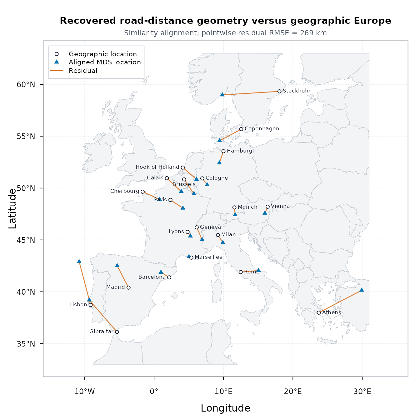
Map of Europe comparing the geographic and similarity-aligned metric MDS locations of 21 cities. Black open circles mark geographic locations, blue triangles mark aligned MDS locations, and orange segments show pointwise discrepancies; the residual RMSE is about 269 kilometres.

The invariance holds at the objective level. The hidden check below translates, rotates, and reflects the returned configuration and verifies that stress is unchanged to numerical tolerance.

Starting from road distances alone, the optimizer recovers a recognizable geometry even though its coordinate frame is arbitrary. The closure and combined-callback pattern used here also applies whenever an objective and gradient share fixed data or an expensive intermediate calculation; ?mize describes the full callback contract.

James Melville

Stress and its gradient

Validate the gradient

Optimize with separate and combined callbacks

Put the configuration on the map

See also