Choosing methods and tuning

James Melville

This guide helps you decide whether a concrete problem or diagnostic justifies changing the default optimizer. Start with Getting started for a first optimization, then return here to choose a direction method, investigate a line search, or run a controlled experiment with a specialized update.

Start here

For a smooth objective with an analytic gradient, begin with the default "L-BFGS" method and line search. It builds a limited-memory curvature model, so it is a useful baseline across a wide range of problem sizes. Record the metric that matters for your application—such as callback count, elapsed time, or objective value at a fixed budget—before comparing alternatives.

Before changing the method

Check the problem setup and the evidence first:

• Validate the analytic gradient at representative points.
• Examine parameter and objective scaling.
• Distinguish an expensive line search from a failed search by inspecting its diagnostic fields.
• Confirm that memory or derivative availability is the actual constraint.
• Decide whether the comparison concerns iterations, callbacks, elapsed time, best objective, or the final iterate.

These checks often identify a local tuning problem without changing the direction method. The Convergence guide explains how stopping rules and budgets affect the result being compared.

Change the direction method when

Method	Consider it when	Main trade-off or diagnostic
"L-BFGS"	You need a general smooth-problem baseline	memory trades curvature history for storage
"BFGS"	Dense state is affordable	Inverse-Hessian storage is quadratic in the parameter count
"SR1"	You want a dense alternative to BFGS	Safeguards may fall back to BFGS or steepest descent
"NEWTON"	A reliable Hessian or inverse Hessian is available	Construction and factorization can dominate; inspect direction_reason after a fallback
"TN"	The problem is large and Hessian-free inner work is acceptable	Gradient differences drive an iterative inner solve
"CG"	Low storage matters and you can tune a nonlinear-CG configuration	Update choice, scaling, and line-search behavior all matter
"SD"	You need a baseline or know a suitable learning rate	Progress depends strongly on the step-size strategy
"NAG" or "Momentum"	Momentum behavior is the subject of the experiment	Define a schedule and compare nonmonotone trajectories explicitly
"DBD"	You want a per-coordinate adaptive learning-rate experiment	Its update controls both direction scaling and step size

"PHESS" reuses a partial-Hessian factorization when fg$hs is available. It remains experimental/internal, so it is documented for completeness rather than recommended as a normal starting point. For algorithmic background on the general direction methods, see Nocedal and Wright.

When supplied curvature is expensive, compare nh and nhi alongside nf and ng. The first pair count accepted fg$hs and fg$hi callback results; they do not count the internal updates used to construct BFGS, SR1, or L-BFGS approximations. This keeps callback cost distinct from algorithmic curvature work. See the mize() result reference for the counting contract and the Convergence guide for its relationship to callback budgets.

Each method-specific control has a fixed scope. For example, memory applies to L-BFGS and to the optional L-BFGS preconditioner for CG or TN; cg_update applies only to CG; and tn_init and tn_exit apply only to TN. Other methods ignore those controls. The same rule applies to step-size controls: DBD ignores line_search, and Wolfe-only controls are ignored by constant and bold-driver steps. See ?mize for the complete accepted values and control scopes.

Tune the line search when

Most methods choose a direction and then use line_search to choose how far to move. With store_progress = TRUE, inspect the diagnostics produced by the search in res$progress. In a stateful loop, the corresponding diagnostics are returned by mize_step_summary(). Start with the field associated with the symptom before changing a control.

Symptom	First evidence to inspect	Possible next action
Many evaluations inside each search	ls_nf, ls_ng, alpha_init, and ls_reason	Revisit scaling, the initial-step rule, or the curvature tolerance
Repeated searches find no usable step	Gradient accuracy, ls_outcome, and direction_reason	Correct the gradient or scaling; then reconsider method/search compatibility
Quasi-Newton steps are repeatedly shortened	Accepted alpha, local model quality, and parameter scaling	Compare try_newton_step policies or rescale the problem
A stable learning rate is already known	Whether a search supplies useful adaptation	Use a constant step in a controlled run
Callback cost must be capped per search	ls_nf, ls_ng, and the global callback totals	Set local search budgets while retaining global hard budgets

Once the diagnostics indicate that the search policy itself is worth changing, the available choices differ in the acceptance conditions and adaptation they provide:

Choice	What it accepts	Useful starting context
"More-Thuente"	Strong Wolfe conditions by default	Default for direction methods, including quasi-Newton and CG
"Rasmussen" or "Schmidt"	Strong Wolfe conditions by default	Alternative Wolfe implementations for comparison or troubleshooting
"Hager-Zhang"	Standard curvature plus approximate Armijo by default	CG-oriented Wolfe search with Hager-Zhang initializers
"Backtracking"	Armijo sufficient decrease	Simpler search when a curvature condition is unnecessary
"Bold Driver"	Any finite objective decrease	Heuristic adaptation from the preceding accepted step
"Constant"	No search; always uses numeric step0	Known learning rate or a controlled experiment

c2, strong_curvature, and approx_armijo apply only to Wolfe searches. c1 also applies to Armijo backtracking. Bold driver and constant steps ignore those controls, and ls_max_alpha and ls_safe_cubic are More-Thuente-specific.

Wolfe conditions and c2

For a direction \(p\), define the line function \(\phi(\alpha) = f(x + \alpha p)\) and assume the initial slope \(\phi'(0) = g(x)^T p\) is negative. Wolfe searches require sufficient decrease and a curvature condition. Under the strong curvature condition,

\[ |\phi'(\alpha)| \leq c_2 |\phi'(0)|. \]

A smaller c2 makes the right-hand side smaller and the condition stricter; a larger c2 makes it looser. The same relationship holds for the standard curvature condition because the initial slope is negative. c2 must lie strictly between c1 and 1.

The CG default is c2 = 0.1. The next comparison changes only c2, holding the start, direction update, line search, initializer, and four-iteration budget fixed. Proposed and selected step lengths show how the search responded; local work reports function and gradient callbacks owned by that outer search.

c2_runs <- lapply(c(`0.1` = 0.1, `0.5` = 0.5), function(c2_value) {
  mize(
    rb0,
    rb_fg,
    method = "CG",
    cg_update = "HZ+",
    line_search = "More-Thuente",
    c2 = c2_value,
    step_next_init = "hz",
    max_iter = 4,
    abs_tol = NULL,
    rel_tol = NULL,
    grad_tol = NULL,
    ginf_tol = NULL,
    step_tol = NULL,
    store_progress = TRUE
  )
})

c2_diagnostics <- do.call(rbind, lapply(seq_along(c2_runs), function(i) {
  progress <- c2_runs[[i]]$progress
  progress <- progress[!is.na(progress$ls_reason), , drop = FALSE]
  data.frame(
    `c2` = names(c2_runs)[i],
    Iteration = seq_len(nrow(progress)),
    `Proposed alpha` = progress$alpha_init,
    `Selected alpha` = progress$alpha,
    `Reason / outcome` = paste(progress$ls_reason, progress$ls_outcome, sep = " / "),
    `Local work (fn / gr)` = paste(progress$ls_nf, progress$ls_ng, sep = " / "),
    check.names = FALSE
  )
}))
rownames(c2_diagnostics) <- NULL
c2_display <- c2_diagnostics
c2_display[["Proposed alpha"]] <- formatC(
  c2_display[["Proposed alpha"]],
  format = "g",
  digits = 4
)
c2_display[["Selected alpha"]] <- formatC(
  c2_display[["Selected alpha"]],
  format = "g",
  digits = 4
)
knitr::kable(c2_display)

c2	Iteration	Proposed alpha	Selected alpha	Reason / outcome	Local work (fn / gr)
0.1	1	1.844e-05	0.0007904	wolfe / wolfe	4 / 4
0.1	2	0.002945	0.002945	wolfe / wolfe	2 / 1
0.1	3	1.245	0.07751	wolfe / wolfe	6 / 5
0.1	4	0.155	0.001196	wolfe / wolfe	6 / 5
0.5	1	1.844e-05	0.0003873	wolfe / wolfe	3 / 3
0.5	2	0.0003956	0.0003956	wolfe / wolfe	2 / 1
0.5	3	0.000479	0.000479	wolfe / wolfe	2 / 1
0.5	4	0.148	0.494	wolfe / wolfe	5 / 4

For this run, changing the curvature tolerance changes accepted step lengths and callback work. ls_reason records why a search stopped, while ls_outcome classifies the point it selected; the two fields answer different diagnostic questions. The callback counts exclude the cached starting point and belong only to the current outer line search.

More-Thuente, Rasmussen, and Schmidt use strong curvature with the exact Armijo condition by default. Hager-Zhang uses the standard curvature condition with the approximate Armijo condition by default. strong_curvature and approx_armijo can override those choices. Such an override changes the conditions whose theory applies, so make it an explicit part of the experiment.

Initial step estimates

Leave the initializer defaults in place unless diagnostics show repeated poor proposals or you need to reproduce another implementation. Hager-Zhang uses its own first-step estimator by default; the other gradient searches default to Rasmussen. A positive finite numeric step0 bypasses the named formulas.

Exact initial-step formulas

On the first outer iteration, the named step0 choices use the starting gradient \(g\) and direction \(p\). Write the directional derivative as \(\phi'(0) = g^T p\).

• "rasmussen": \(1 / (1 - \phi'(0))\). For steepest descent, this becomes \(1 / (1 + \lVert g \rVert_2^2)\).
• "scipy": \(-\lVert g \rVert_2 / \phi'(0)\). For steepest descent, where \(p = -g\), this reduces to \(1 / \lVert g \rVert_2\).
• "schmidt": \(1 / \lVert g \rVert_1\); there is no added 1 in the denominator.
• "hz": Hager-Zhang scaling based first on the relative infinity norms of the parameters and gradient, then on the objective and squared gradient norm, with a safeguarded fallback.

After the first iteration, step_next_init can use a slope ratio, quadratic interpolation, the Hager-Zhang "hz" rule, or a fixed positive number. The Hager-Zhang rule may make one objective-only probe to fit a quadratic. It does so only when a previous step exists and both the local line-search budgets and the remaining hard budgets leave room for the probe and a subsequent search. Otherwise it falls back to an enlarged, safeguarded version of the previous step. A probe is included in ls_nf.

try_newton_step adjusts a calculated proposal upward, at most to the natural unit step of 1. Its current default is TRUE for "NEWTON", "PHESS", "BFGS", "SR1", "L-BFGS", and "TN", and FALSE otherwise. Set it explicitly when comparing initialization policies.

Backtracking, constant, and bold-driver steps

Armijo backtracking repeatedly reduces the candidate until it provides the decrease controlled by c1. With step_down = NULL, the implementation uses cubic interpolation and evaluates function and gradient at candidate points. A numeric step_down instead multiplies the candidate by that factor and uses function-only candidate evaluations.

backtracking_res <- mize(
  rb0,
  rb_fg,
  method = "SD",
  line_search = "Backtracking",
  step0 = 1,
  step_down = 0.5,
  max_iter = 10
)

constant_res <- mize(
  rb0,
  rb_fg,
  method = "SD",
  line_search = "Constant",
  norm_direction = TRUE,
  step0 = 0.01,
  max_iter = 10
)

bold_res <- mize(
  rb0,
  rb_fg,
  method = "SD",
  line_search = "Bold Driver",
  step_down = 0.5,
  step_up = 1.1,
  max_iter = 10
)

The constant strategy requires a numeric step0 and performs no search. With steepest descent, norm_direction = TRUE makes step0 the parameter-update length directly.

Bold driver accepts the first tested point with a lower objective, reduces failed proposals by step_down, and initializes the next iteration by multiplying the last accepted step by step_up. Its first proposal is 1; step0, c1, c2, and step_up_fun do not configure that proposal. ls_max_fn is its local callback limit. Stored progress reports objective_decrease when it accepts a point and no_step with the reason when it cannot make a usable change. A zero Bold Driver sub-step does not cancel a nonzero update from a later momentum stage; it becomes a line-search failure only when the complete optimizer step is also zero.

For Wolfe and backtracking searches, ls_max_fn, ls_max_gr, and ls_max_fg limit callbacks within one outer line search. The optimizer budgets max_fn, max_gr, and max_fg remain hard limits for the entire run. See the line-search reference for specialized safeguards and defaults.

Momentum and adaptive learning-rate methods

The trajectory comparisons below use a fixed outer-iteration budget. abs_tol = 0 asks the high-level loop to observe the objective at every iteration so the tables and plots describe the accepted trajectory; the other ordinary tolerances are disabled. They illustrate one problem and do not establish convergence or a generally superior configuration. Comparison tables report both best and last objectives because momentum trajectories may be nonmonotone.

Nesterov Accelerated Gradient ("NAG")

NAG takes a steepest-descent step and then applies a momentum update. Its current objective can increase on an iteration, so inspect the full trajectory and the returned best result.

nest_q controls the "nsconvex" NAG schedule. It ranges from 0, the non-strongly-convex limit and largest momentum, to 1, zero momentum. The default is 0. With nest_q = 1 and nest_convex_approx = FALSE, callback counts match method = "SD" and progress data have no mu column.

nag_runs <- list(
  `q = 0` = run_bounded("NAG", nest_q = 0),
  `q = 0.001` = run_bounded("NAG", nest_q = 0.001)
)
assert_bounded_runs(nag_runs)
knitr::kable(summarize_runs(nag_runs), digits = 6)

Run	Best objective	Last objective	Function callbacks	Gradient callbacks	Status	Termination
q = 0	1.054056	6.055306	994	993	budget_exhausted	max_iter
q = 0.001	1.147505	2.765938	835	834	budget_exhausted	max_iter

plot_current_objective(nag_runs)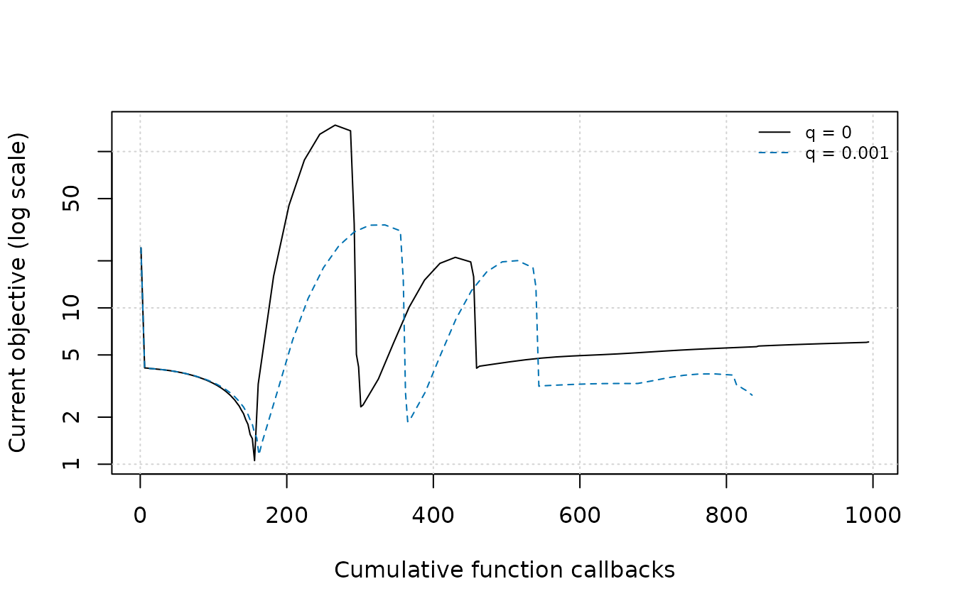

Current objective against cumulative function callbacks for two NAG schedules. Both runs use the same start and fixed 100-iteration budget.

The objective paths are nonmonotone, so the final value does not summarize every iterate a run visited. Choose either the best or last objective before the comparison and use that metric consistently.

The theoretical step-size and momentum guarantees require assumptions and problem constants that this Rosenbrock example does not supply. For derivations and historical context, see the Nesterov background note.

Momentum schedules and update order

With method = "Momentum", mom_schedule defines the momentum fraction:

Value	Schedule
A finite number such as 0.9	Constant momentum
"switch"	Change from finite mom_init to finite mom_final at mom_switch_iter
"ramp"	Increase linearly from finite mom_init to finite mom_final
"nsconvex"	Use the NAG schedule, controlled by the nest_* arguments
A function	Compute a finite numeric scalar from the iteration, optionally also max_iter

Numeric schedule values and function results are clamped to the interval [0, 1]. The "switch" and "ramp" schedules require both mom_init and mom_final.

A deterministic custom schedule is easiest to inspect independently of an optimizer trajectory:

cosine_schedule <- function(iter, max_iter) {
  phase <- min(iter / max_iter, 1)
  0.4 + 0.2 * (1 - cos(pi * phase))
}

schedule_values <- data.frame(
  Iteration = c(1, 5, 10),
  Momentum = vapply(
    c(1, 5, 10),
    cosine_schedule,
    numeric(1),
    max_iter = 10
  )
)
knitr::kable(schedule_values, digits = 3)

Iteration	Momentum
1	0.41
5	0.60
10	0.80

The values show the intended smooth increase over the ten-iteration schedule. mize clamps custom schedules to the supported momentum range. Prefer a built-in schedule when it already expresses the intended experiment.

mom_type = "classical" applies momentum after the gradient step; mom_type = "nesterov" applies it before that step. The next comparison holds the schedule, start, objective, and budget fixed.

momentum_runs <- list(
  Classical = run_bounded("Momentum", mom_schedule = 0.9),
  Nesterov = run_bounded(
    "Momentum",
    mom_schedule = 0.9,
    mom_type = "nesterov"
  )
)
assert_bounded_runs(momentum_runs)
knitr::kable(summarize_runs(momentum_runs), digits = 6)

Run	Best objective	Last objective	Function callbacks	Gradient callbacks	Status	Termination
Classical	3.423736	20.331401	1272	1271	budget_exhausted	max_iter
Nesterov	0.353595	0.584473	1088	1087	budget_exhausted	max_iter

plot_current_objective(momentum_runs)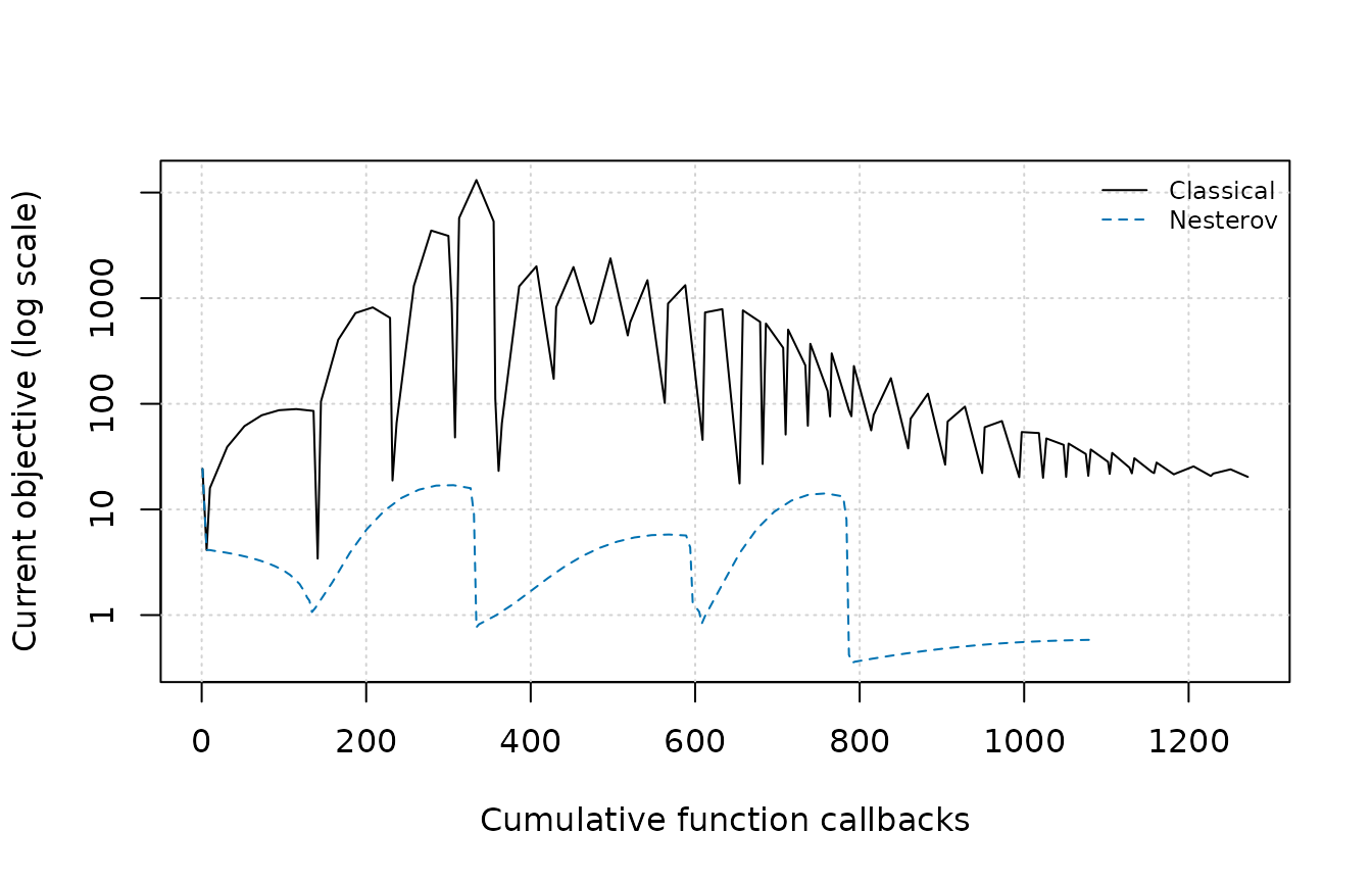

Current objective for classical and Nesterov-style momentum under one fixed schedule and 100-iteration budget.

The table and trajectories show how update order changes this bounded run. Treat both orders as choices to test on the problem at hand. With mom_schedule = "nsconvex", nest_convex_approx = TRUE selects Sutskever’s approximation for the nest_q = 0 case and causes nest_q to be ignored.

Delta-Bar-Delta learning rates

method = "DBD" changes a per-coordinate learning rate according to agreement in sign between the current gradient and a weighted history. Because DBD chooses both direction scaling and step size, it ignores line_search.

The main controls are:

• step0, the initial per-coordinate learning rate;
• step_down, the multiplicative decrease when signs disagree;
• step_up, the increase when signs agree;
• step_up_fun, either "*" for a proportional increase or "+" for an additive increase; and
• dbd_weight, the gradient-history weight when no momentum schedule is used.

step0 must be a positive finite numeric scalar or one of the named first-step initializers described above. Named estimates are safeguarded before DBD uses them, and the "hz" estimate uses the current parameter scale.

The following configuration uses the additive update associated with the t-SNE-style variant. It demonstrates control semantics; adopting it for a smooth optimization problem requires problem-specific evidence.

dbd_res <- mize(
  rb0,
  rb_fg,
  method = "DBD",
  step0 = "rasmussen",
  step_down = 0.8,
  step_up = 0.2,
  step_up_fun = "+",
  dbd_weight = 0.5,
  max_iter = 10
)

If a momentum schedule is supplied with DBD, dbd_weight is ignored and the momentum update supplies the history. mom_type selects classical or Nesterov update ordering, as it does for method = "Momentum". DBD’s step calculation is gradient-based, although function-based convergence criteria and best-result reporting may still request objective evaluations. Budget explicitly for the observations selected by the convergence controls.

Adaptive restart

O’Donoghue and Candes proposed restarting accelerated schemes when momentum appears unhelpful. A restart discards the stored momentum update and resets iteration-dependent momentum schedules. In mize, it can be applied to any optimizer configuration that uses momentum.

restart	Trigger
"fn"	The objective does not decrease on consecutive iterations
"gr"	The proposed update is not a descent direction
"speed"	The update vector does not grow in Euclidean norm

Gradient restart is unavailable with mom_type = "nesterov" because its gradient is evaluated at a different location. restart_wait specifies the number of iterations after a restart before another restart is allowed; its default is 10.

The comparison below uses classical momentum and varies only restart type and waiting period. The no-restart result is reused from the preceding comparison.

restart_runs <- list(
  None = momentum_runs[["Classical"]],
  `fn, wait = 10` = run_bounded(
    "Momentum",
    mom_schedule = 0.9,
    restart = "fn",
    restart_wait = 10
  ),
  `gr, wait = 10` = run_bounded(
    "Momentum",
    mom_schedule = 0.9,
    restart = "gr",
    restart_wait = 10
  ),
  `fn, wait = 1` = run_bounded(
    "Momentum",
    mom_schedule = 0.9,
    restart = "fn",
    restart_wait = 1
  ),
  `gr, wait = 1` = run_bounded(
    "Momentum",
    mom_schedule = 0.9,
    restart = "gr",
    restart_wait = 1
  )
)
assert_bounded_runs(restart_runs)
knitr::kable(summarize_runs(restart_runs), digits = 6)

Run	Best objective	Last objective	Function callbacks	Gradient callbacks	Status	Termination
None	3.423736	20.331401	1272	1271	budget_exhausted	max_iter
fn, wait = 10	0.687237	2.964871	1184	1174	budget_exhausted	max_iter
gr, wait = 10	0.687237	2.964871	1175	1174	budget_exhausted	max_iter
fn, wait = 1	0.000175	0.000175	470	461	budget_exhausted	max_iter
gr, wait = 1	0.000097	0.000119	797	796	budget_exhausted	max_iter

plot_current_objective(restart_runs)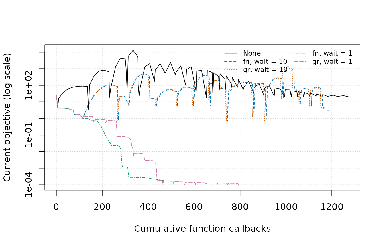

Current objective for classical momentum with no restart and four adaptive-restart configurations under the same 100-iteration budget.

The table places trajectory summaries beside callback demand. Function-based validation may add an objective callback when the value is not cached; gradient validation has the same relationship to available gradients. Compare both callback columns and tune restart policy under the budget and metric that matter for the application.

See also

• Getting started provides the shortest route to a first result.
• Convergence explains the status and termination fields used in every bounded comparison.
• Nesterov accelerated gradient and momentum develops the schedule derivations and historical background.
• Quasi-hyperbolic momentum covers another momentum formulation.