This article retains its original experiments and examples. For current package usage, see the usage guide.
Introduction
Here are some comparisons between PaCMAP and UMAP. None of this will make sense without reading Notes on PaCMAP and maybe PaCMAP Examples.
Images are generated by starting with UMAP and then using
uwot to attempt to get progressively closer to PaCMAP’s
behavior.
Validation
Numerical validation is by:
-
nnp15. Mean 15 nearest neighbor preservation. This is always the exact 15 nearest neighbors in the input space before any PCA, so potentially methods that use PCA and the local scaling of nearest neighbors are at a slight disadvantage. -
nnp65. Mean 65 nearest neighbor preservation. For local scaled neighbors, this is the number of neighbors the 15 neighbors are chosen from. -
rtp. Random triplet preservation with 20 triplets per observation. The favored global structure preservation method of the PaCMAP paper. Random initialization gives a value of0.5. -
dcorr. The Pearson correlation between 100,000 pairwise distances sampled at random. Random initialization gives a value of0. Related to a measure of global structure used by Becht and co-workers. -
emd. Earth mover’s distance based on 100,000 pairwise distances sampled randomly. Based on work by Heiser and Lau I am a bit skeptical of the use of this method due to the form of normalization. The problem manifests particularly with random initialization not giving consistent results. It depends on the initial standard deviation, whether a normal or uniform random distribution is used and the identity of the dataset itself. Worse, for a large number of datasets here, the plain PCA initialization gives a larger EMD than the UMAP-style random initialization. Formnist, the PCA result has a larger EMD than even a t-SNE style random initialization (normal distribution with a standard deviation of0.0001).
These numbers are usually fairly stable between runs of the embedding
algorithms with different random number seeds (and sampling variance for
rtp, dcorr and emd) to 0.01 or
0.02. Differences larger than that may therefore indicate a proper
difference between methods (whether you consider it practically
significant or not is another matter). coil20 seems to be
the “twitchiest” of the datasets for this and can show larger changes in
dcorr (0.05-0.1) even between runs of PaCMAP (which is a
shame as PaCMAP tries to reduce such variability). I suspect this is
because the number of neighbors is too low for a good global layout: the
high dimensional graph is not fully connected. You’d hope the mid-near
pair business would help here, but the clusters do re-arrange themselves
from run to run.
Other datasets which aren’t fully connected with
n_neighbors = 15 (with exact nearest neighbors) are:
iris, coil100, tasic2018 and
norb.
Results
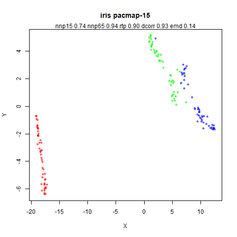
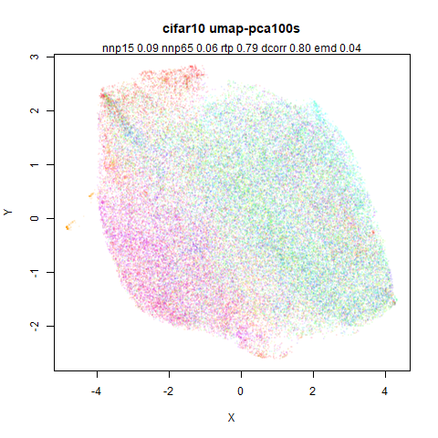
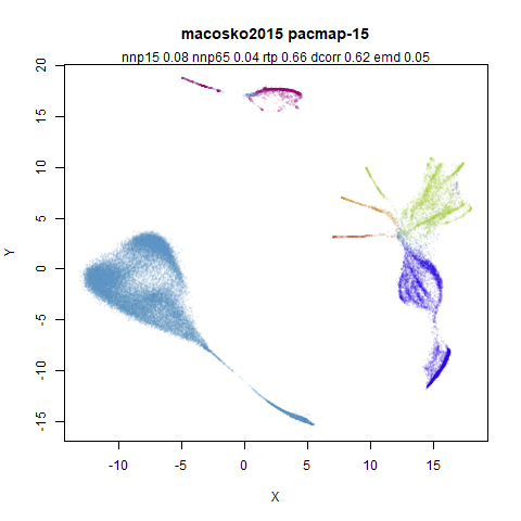
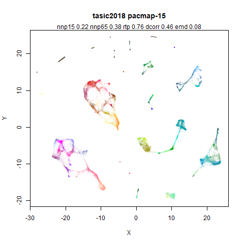
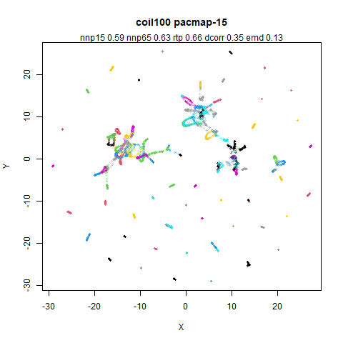
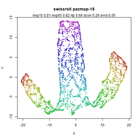
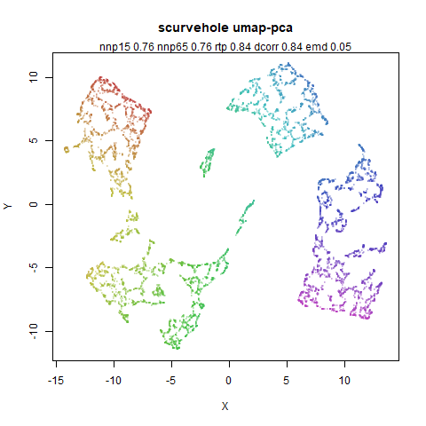
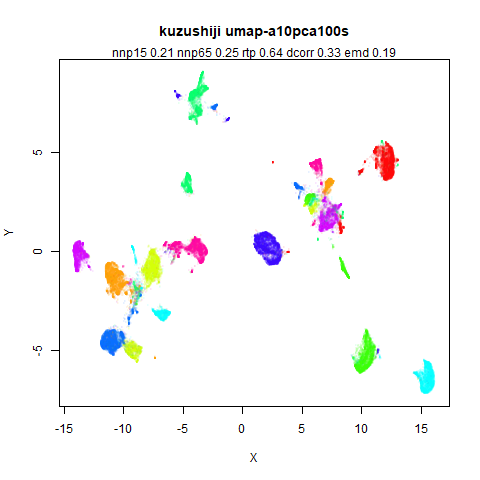
- Top left: PaCMAP using 15 nearest neighbors for all datasets. Defaults otherwise.
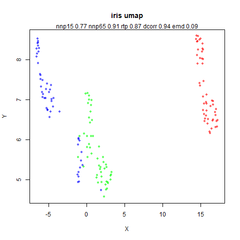
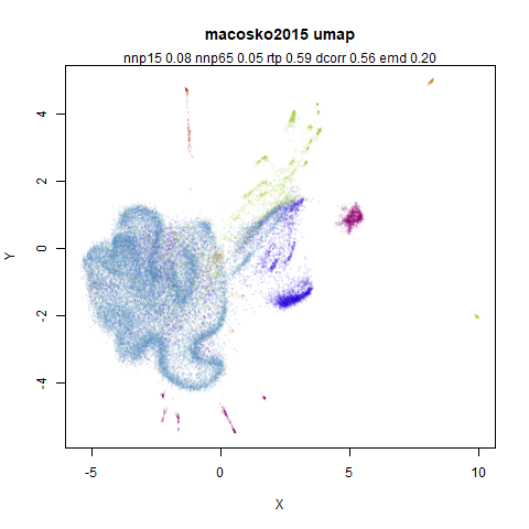
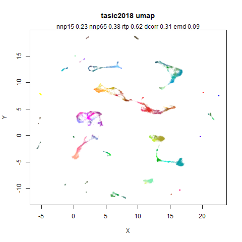
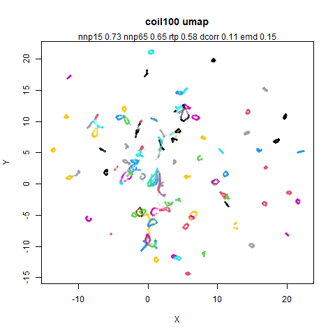
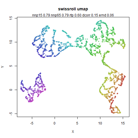
- Top right: UMAP (via the Python
umap-learn) with defaults. - Middle left: UMAP (via
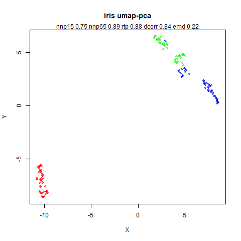
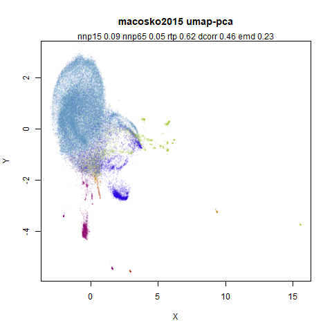
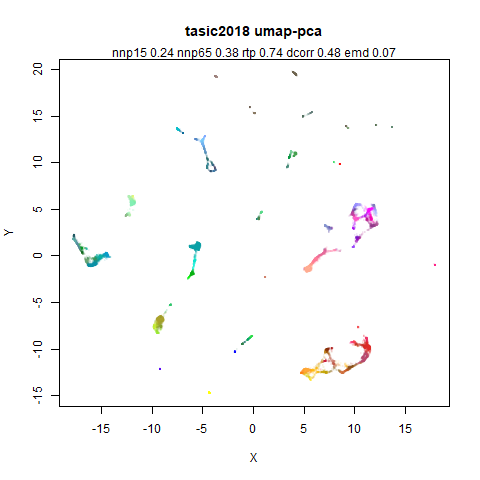
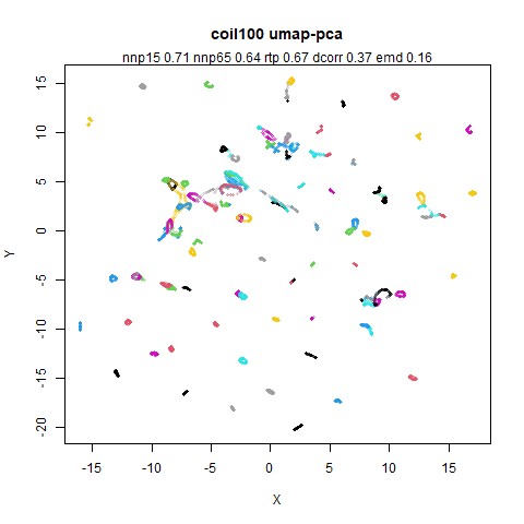
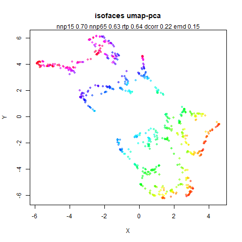
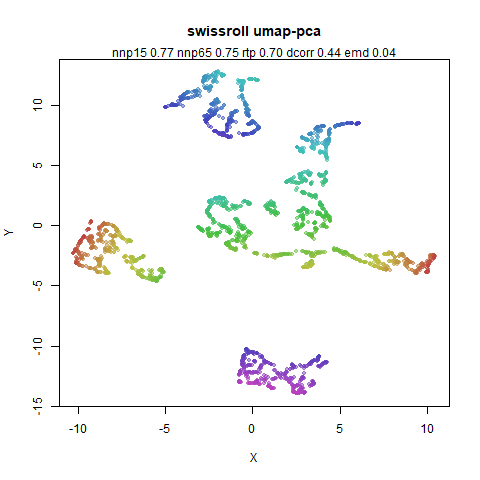
uwot) with a PCA initialization and the standard deviation scaled to 1 for both dimensions. We expect initialization to be important for the results, so replacing UMAP’s spectral initialization with a PCA initialization should be informative. Also the PaCMAP’s paper observes the scale invariance of initialization in methods like UMAP to motivate the use of mid-near pairs. What if we control the initial scale of the PCA, in this case withinit_sdev = 1? - Middle right: UMAP (again via
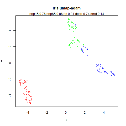
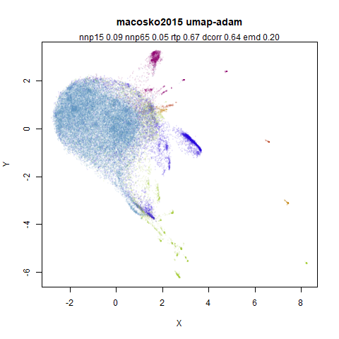
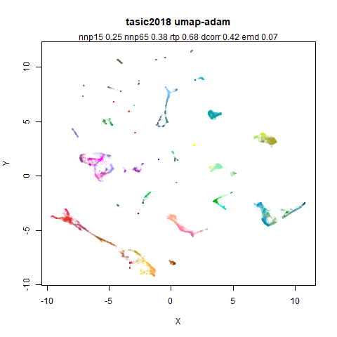
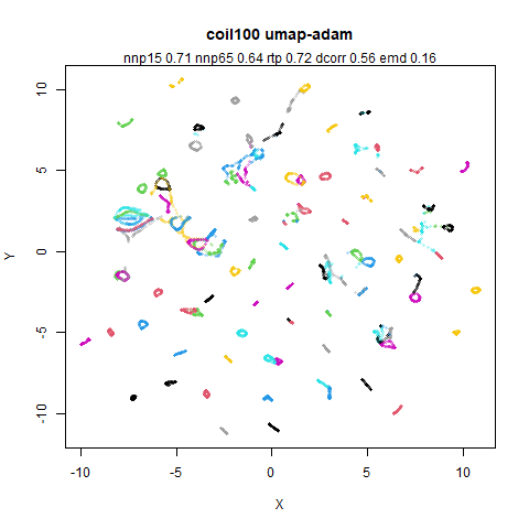
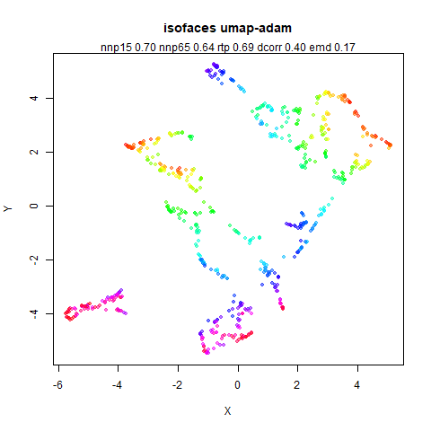
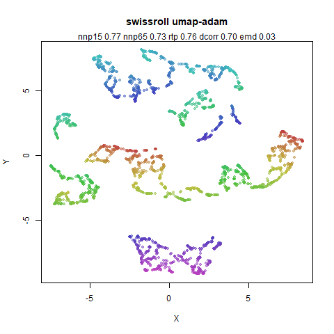
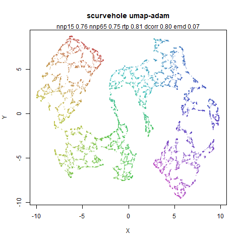
uwot) with the same PCA initialization but also switching from the stochastic gradient descent optimization to the batched Adam optimization method used by PaCMAP. Also the same number of iterations are used for all datasets (n_epochs = 450) to match that done by PaCMAP. - Bottom left: UMAP (via
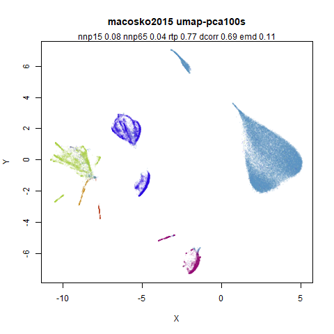
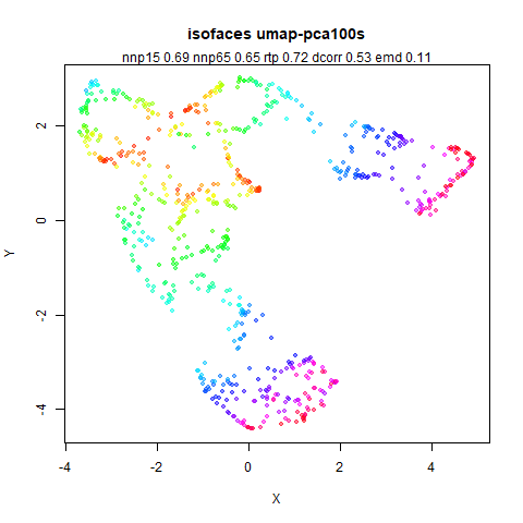
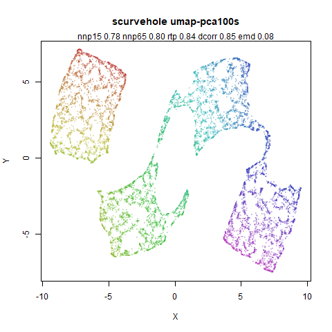
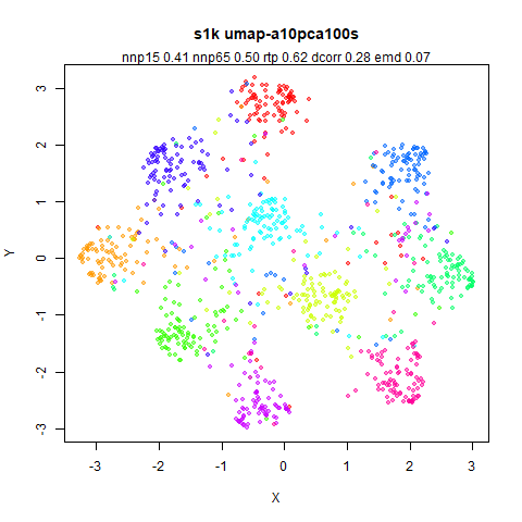
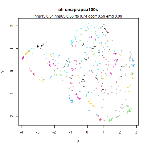
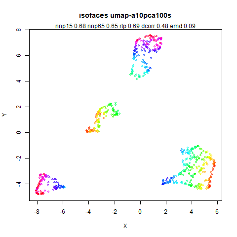
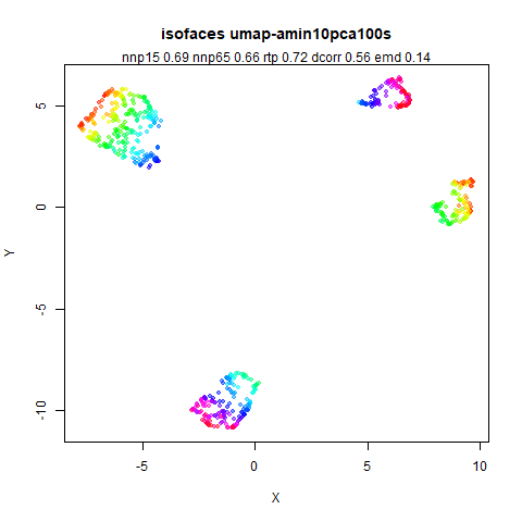
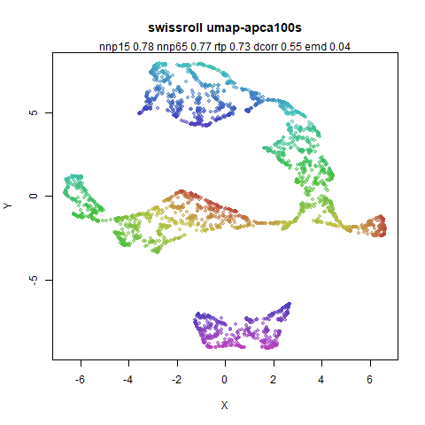
uwot), PCA initialization, Adam optimization and use binary edge weights like PaCMAP, and use PaCMAP’s scaled nearest neighbors approach for near pairs. Also for datasets that have an input dimensionality of 100, reduce to 100 via PCA, the PaCMAP default. For some datasets the PCA reduction has no effect other than speeding up the nearest neighbor search, but for others it can have a bigger effect. - Bottom right: UMAP (via
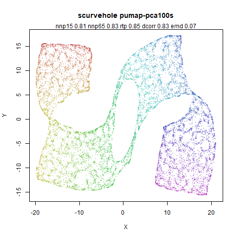
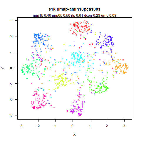
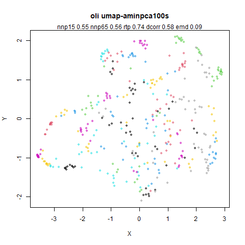
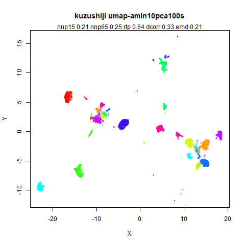
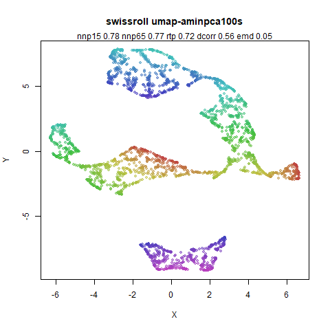
uwot), PCA initialization, Adam optimization, locally scaled nearest neighbor selection, PCA reduction to 100 dimensions, binary edge weights and using the PaCMAP near pair and far-pair forces rather than UMAP’s attractive and repulsive interactions. This is as close asuwotcan get to PaCMAP behavior without adding the mid-near pairs.
iris
 |
 |
 |
 |
 |
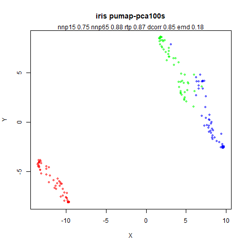 |
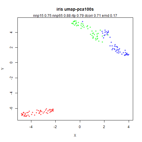
In my experience iris rarely behaves like other
datasets, but there’s no reason to not try it out. PaCMAP’s
nnp15 is the lowest, but its nnp65 is the
highest. The rtp is also highest for PaCMAP. Adding more
and more PaCMAP-like behavior to UMAP doesn’t help until the PaCMAP
attractive force replaces UMAP. But also bear in mind that visually
there is hardly a huge difference.
s1k
 |
 |
 |
 |
 |
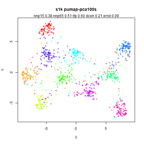 |
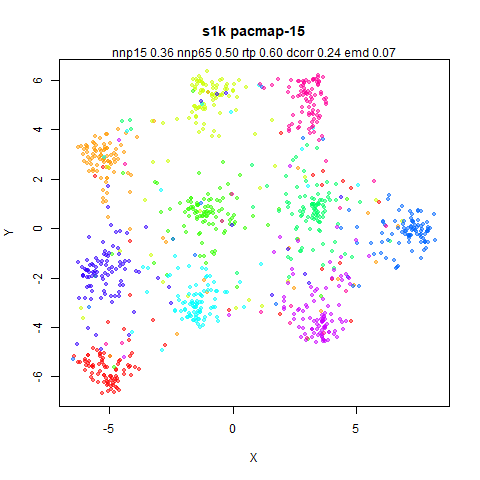
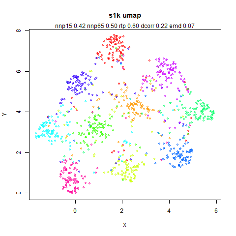
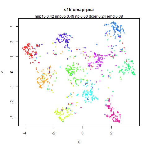
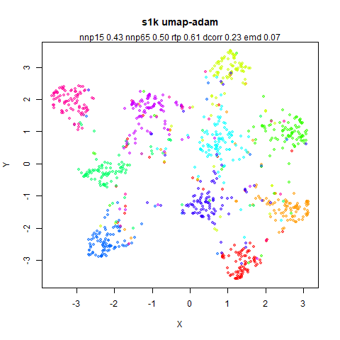
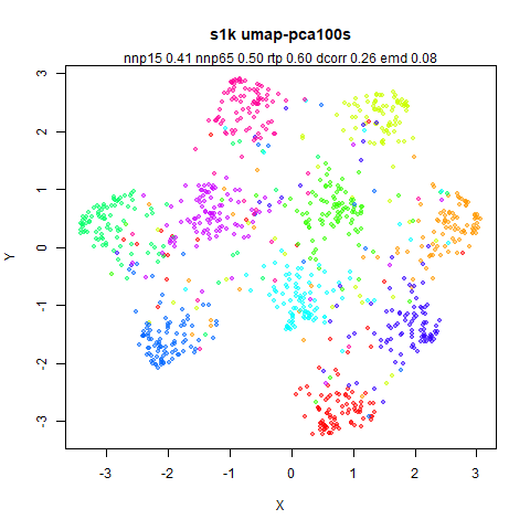
UMAP has a superior nnp15 compared to PaCMAP (it’s
telling that adding the PaCMAP attractive force in going from the bottom
left to bottom right image causes the nnp15 to drop), but
the nnp65 is very stable. rtp is also stable
for every method.
oli
 |
 |
 |
 |
 |
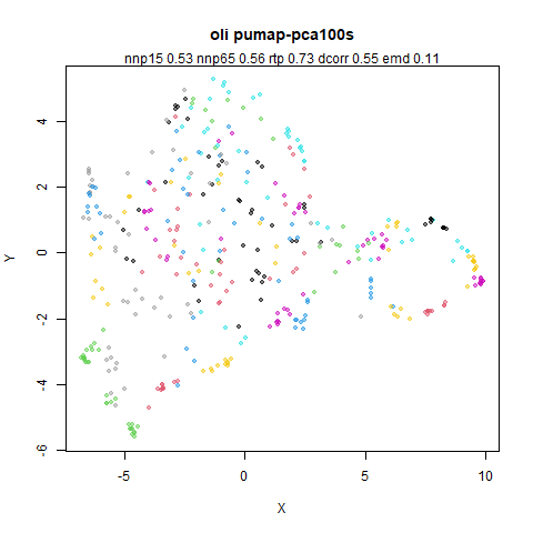 |
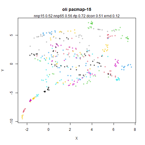
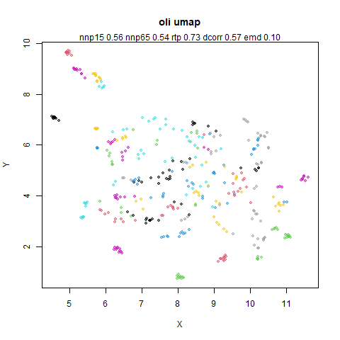
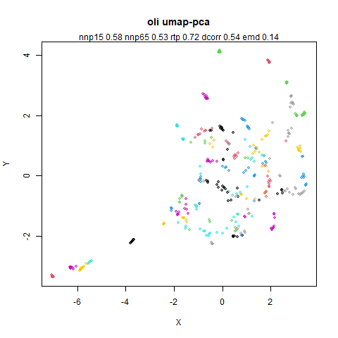
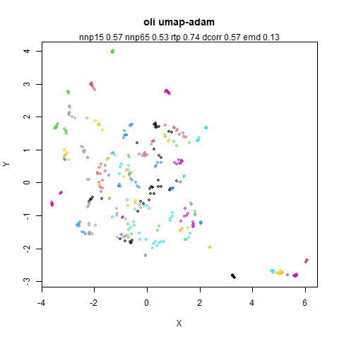
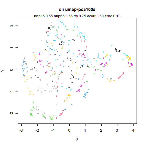
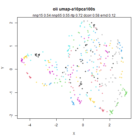
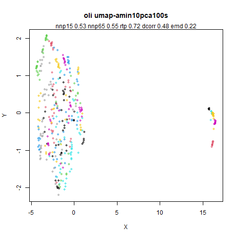
Very little to choose from any method here. The bottom row indicates that the difference between the UMAP and PaCMAP attractive forces is very minor for this dataset.
frey
 |
 |
 |
 |
 |
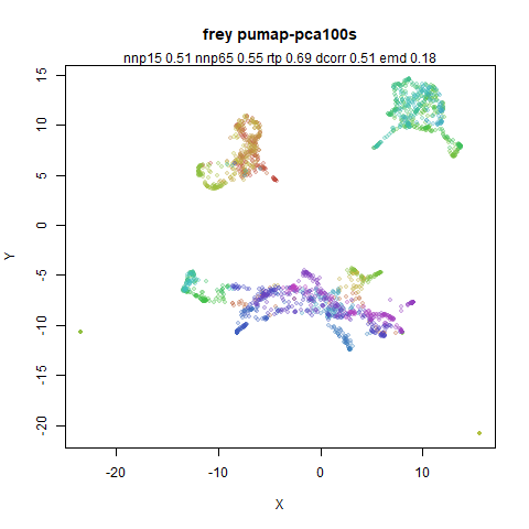 |
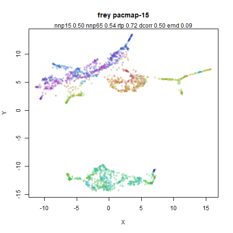
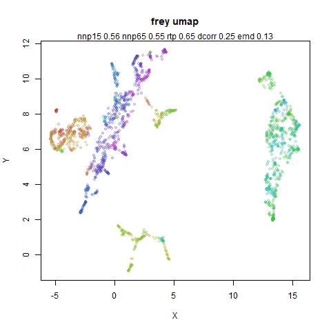
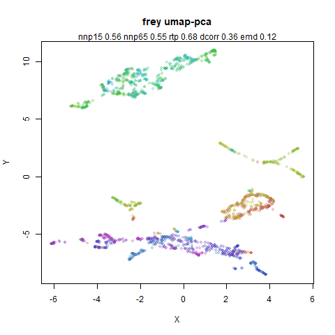
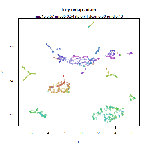
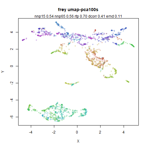
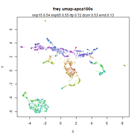
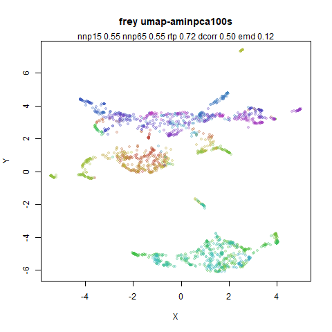
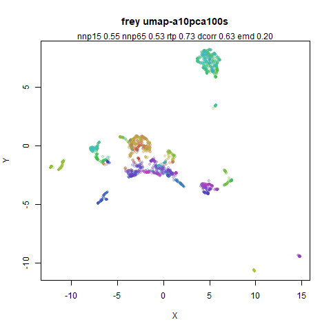
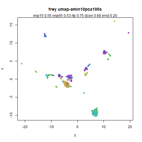
I have come to expect that the frey faces results are
often all over the place and so it is here. nnp65 holds up
across all methods, but visually there is quite a bit of variation. UMAP
dcorr results are much lower than for PaCMAP and just
initializing from PCA only closes around half the gap. But then
optimizing with Adam produces the best dcorr and
rtp. Visually don’t know if I like it though: it seems to
have split some of the manifold into larger pieces.
coil20
 |
 |
 |
 |
 |
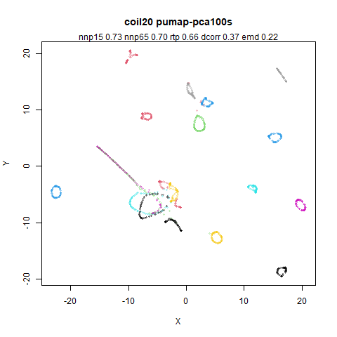 |
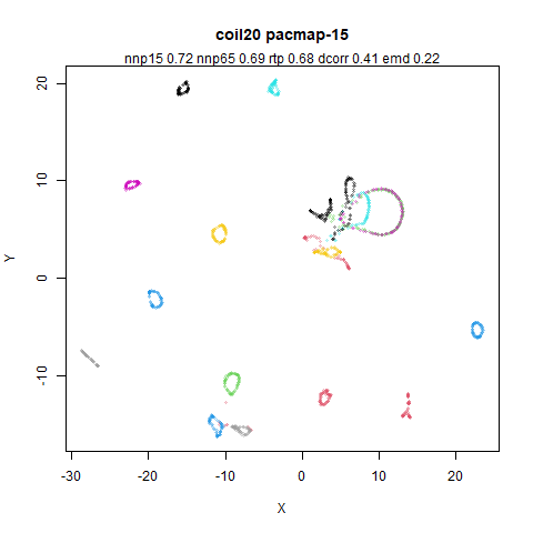
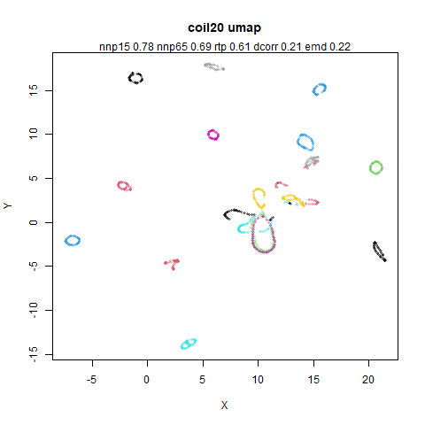
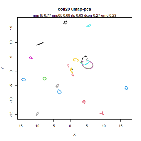
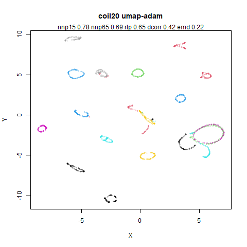
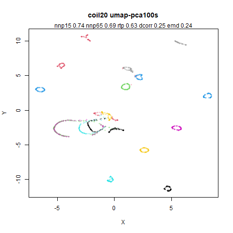
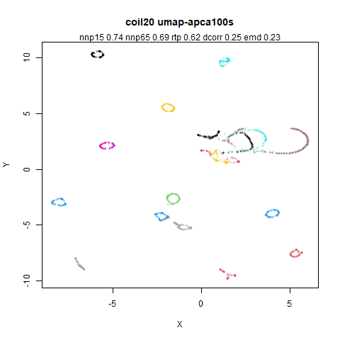
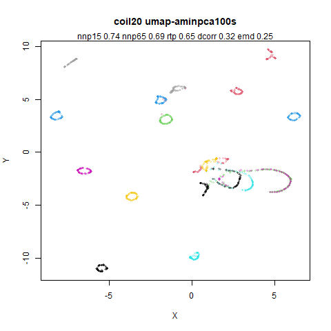
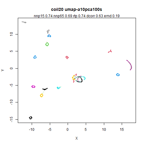
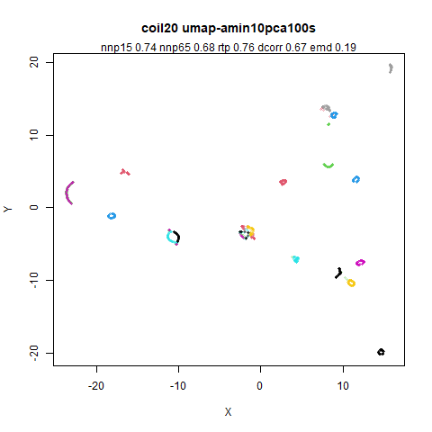
coil20 behaves rather like frey: UMAP does
badly in terms of dcorr until Adam is added as the
optimizer, and then adding the binarized edge weights seems to
negatively affect the dcorr. rtp seems less
affected though.
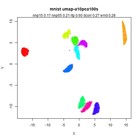
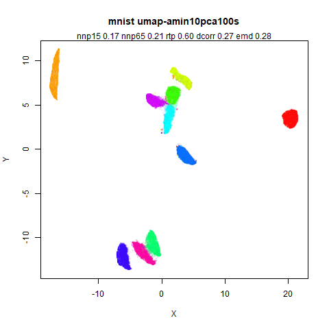
mnist
 |
 |
 |
 |
 |
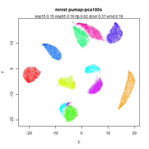 |
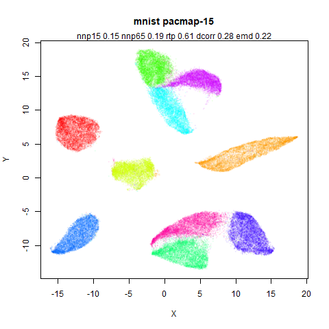
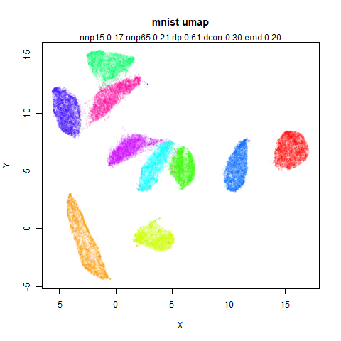
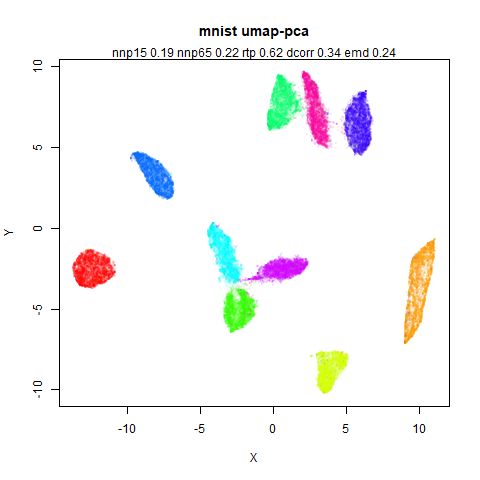
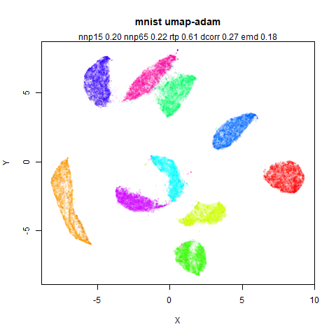
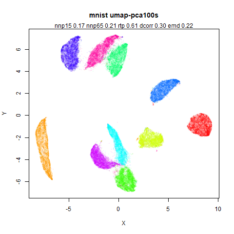
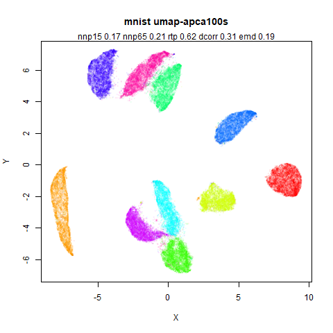
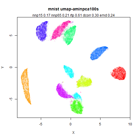
Clusters move about a bit quite a lot across the different runs.
Notably where the 3 (green), 5 (cyan) and 8 (magenta) clusters are
usually together, when Adam is the optimizer, the 2 cluster (yellow) has
got between the 3 cluster (green) and the 5+8 cluster. When the PaCMAP
attractive forces are used in uwot, the 8 cluster is on its
own, but a small part of it can be seen still with the 3+5 clusters.
None of the metrics really help with detecting any of this, though.
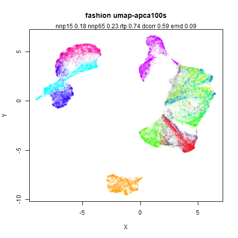
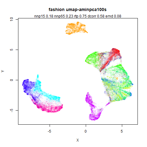
fashion
 |
 |
 |
 |
 |
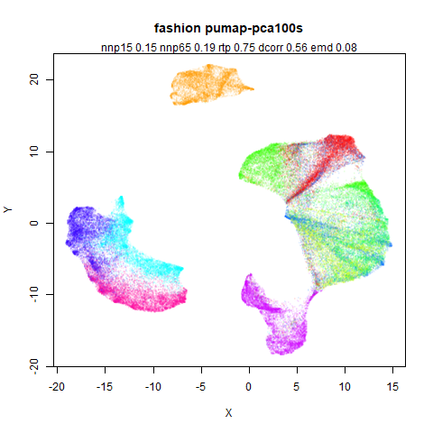 |
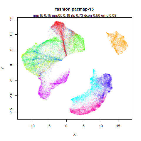
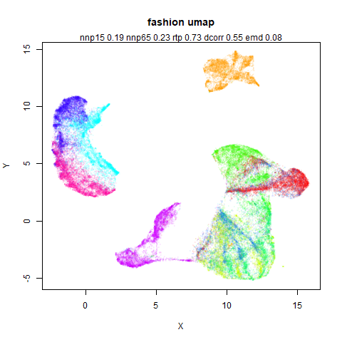
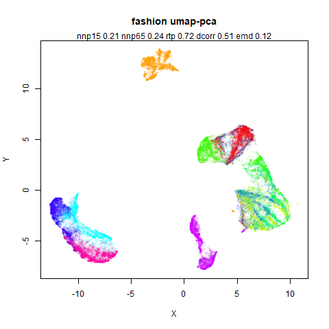
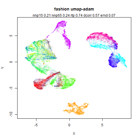
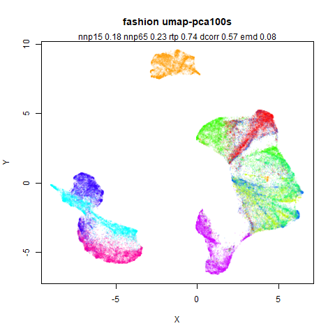
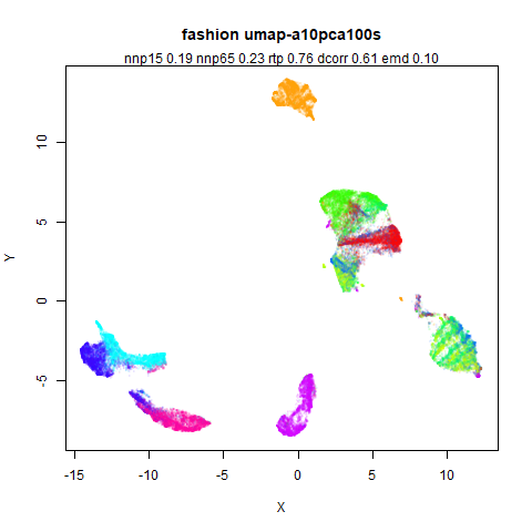
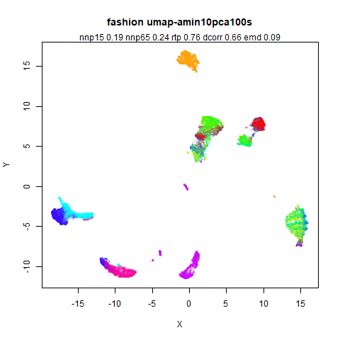
UMAP seems to do better at the nnp65 local preservation.
UMAP with the PCA initialization sees a mild drop in dcorr,
but not for rtp and then it jumps back up with the Adam
optimization.
kuzushiji
 |
 |
 |
 |
 |
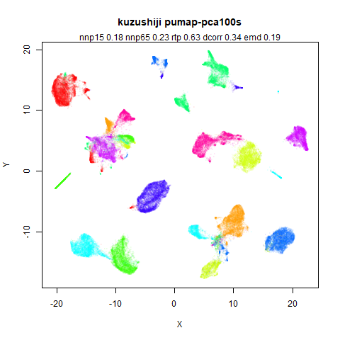 |
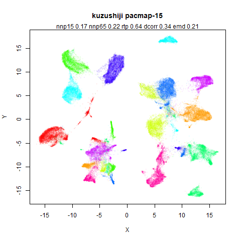
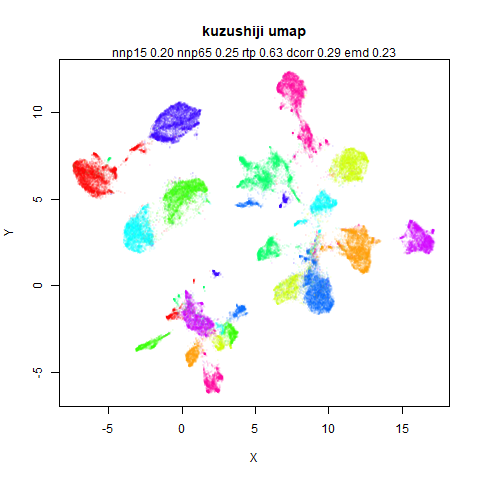
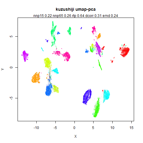
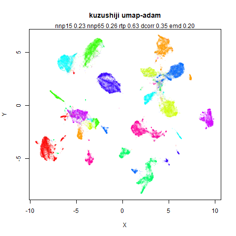
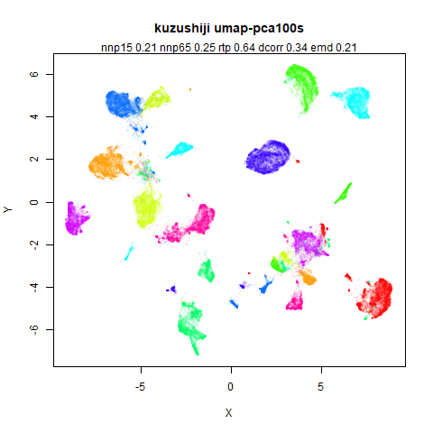
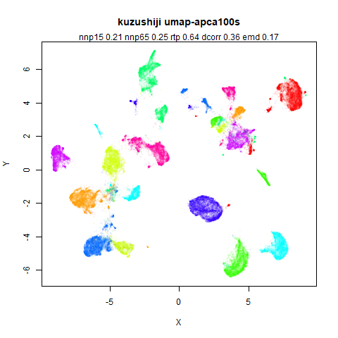
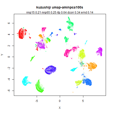
This is another case where visually the clusters seem to settle into different arrangements but the metrics don’t reflect large changes.
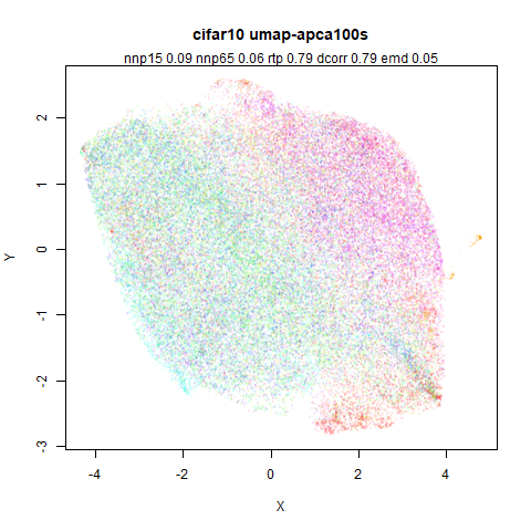
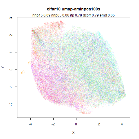
cifar10
 |
 |
 |
 |
 |
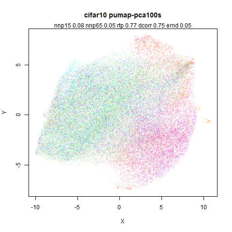 |
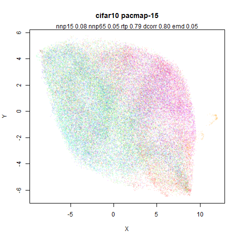
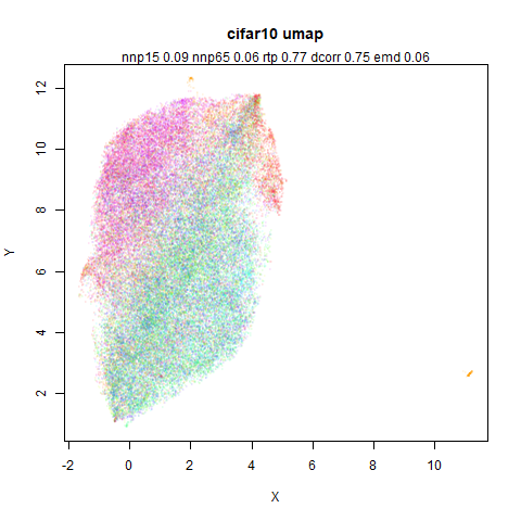
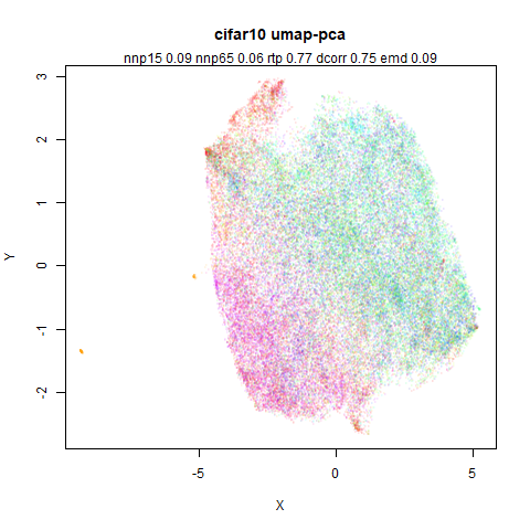
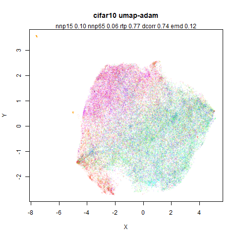
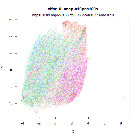
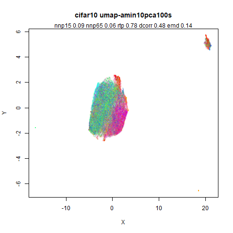
This is not a dataset that seems amenable to good separation of clusters, at least by using Euclidean distance on the raw pixel values.
macosko2015
 |
 |
 |
 |
 |
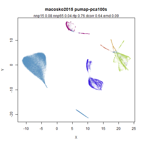 |
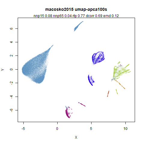
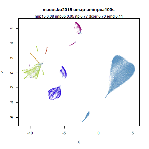
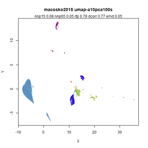
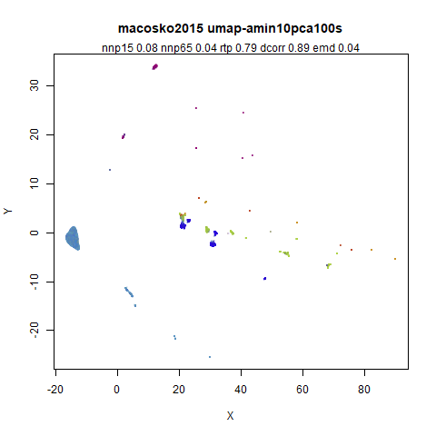
It is immediately obvious that PCA has a huge effect on the display
of this data. And yet local preservation is unchanged (and pretty
crummy) either way. But the rtp actually goes up and UMAP
outperforms PaCMAP.
tasic2018
 |
 |
 |
 |
 |
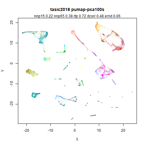 |
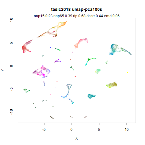
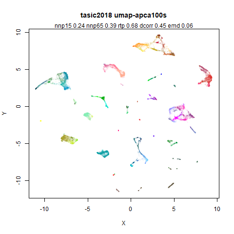
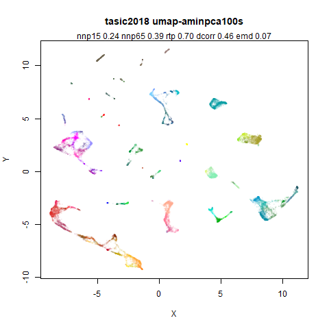
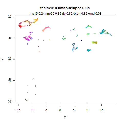
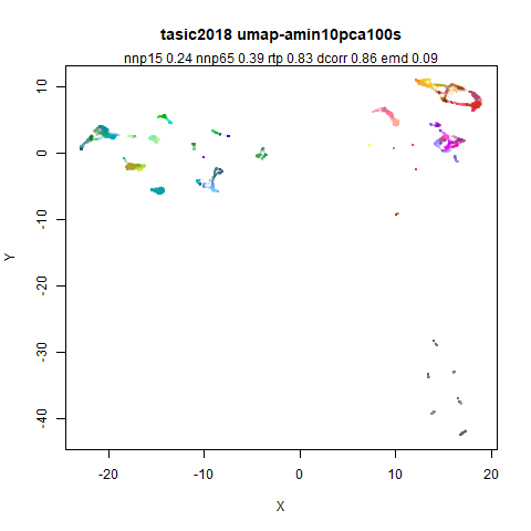
rtp and dcorr seems to favor PaCMAP here.
Some combination of the PaCMAP attractive forces and PCA initialization
seems to be key.
mammoth
 |
 |
 |
 |
 |
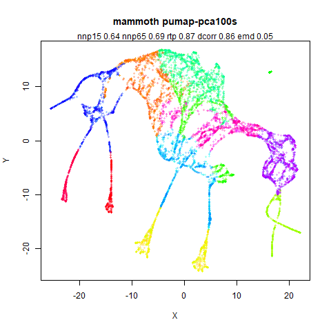 |
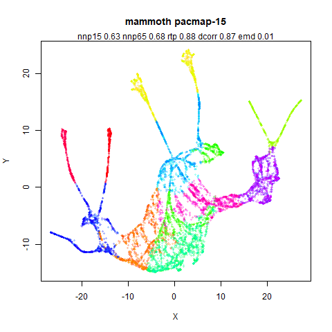
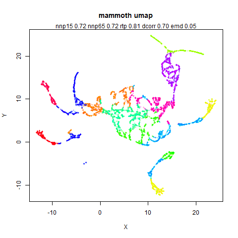
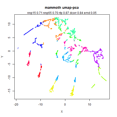
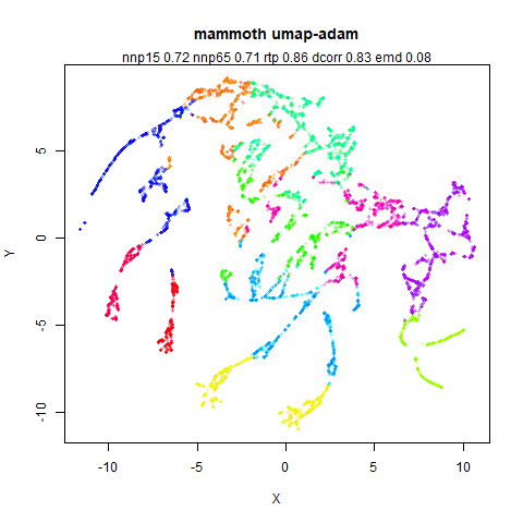
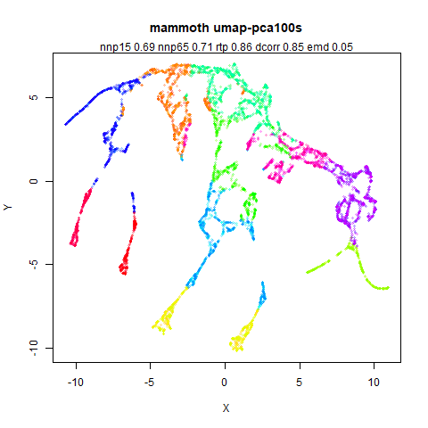
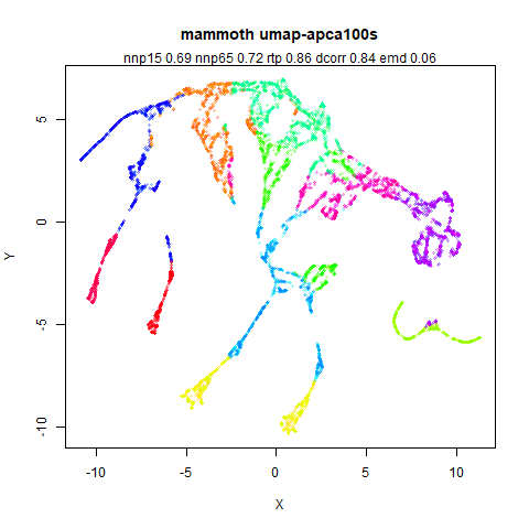
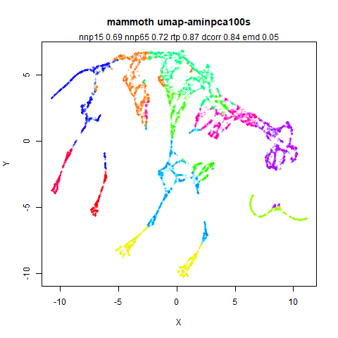
UMAP definitely breaks up the mammoth structure into false clusters
here, and PCA initialization seems definitely superior to spectral
initialization in terms of rtp and dcorr.
Binarizing the edge weights (going from the image middle right to bottom
left) has a visually striking effect, and crossing tusks aside, the
pumap result is nearly as good as the PaCMAP one.
ng20
 |
 |
 |
 |
 |
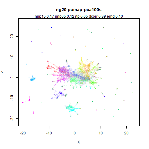 |
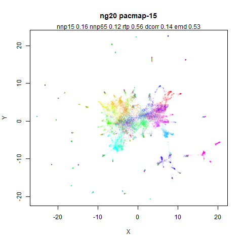
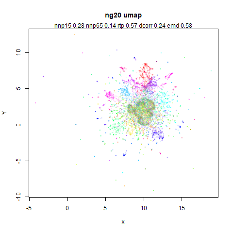
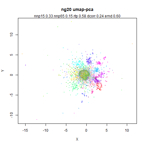
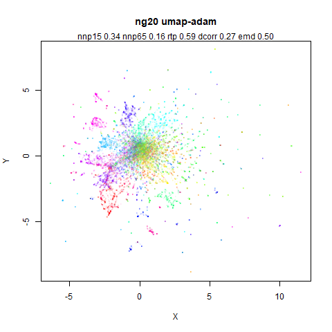
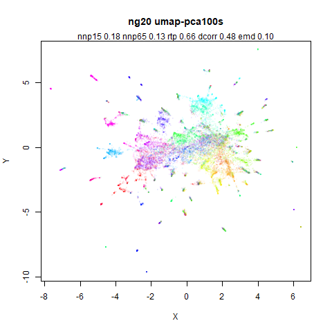
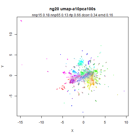
PaCMAP dcorr is poor here. This is another example where
there is a noticeable visual change when the preprocessing with PCA to
100D is used. But that doesn’t seem to be the cause of the lowered
dcorr, as UMAP (bottom left) has the best
dcorr (and rtp) using it. dcorr
drops when PaCMAP forces replace UMAP.
norb
 |
 |
 |
 |
 |
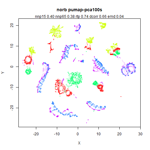 |
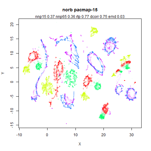
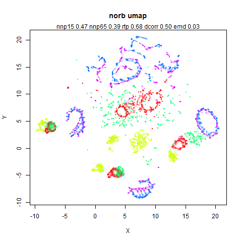
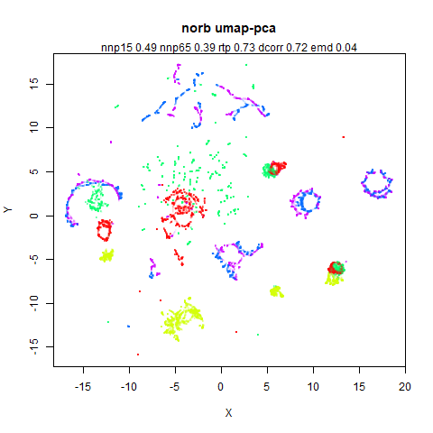
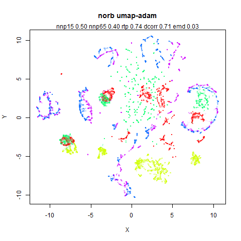
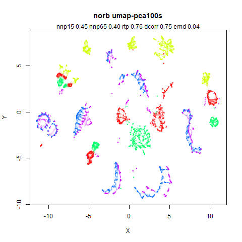
PaCMAP settings do well for this dataset in terms of rtp
and dcorr. UMAP (bottom left) is competitive with it if it
adopts PaCMAP settings and may also do a bit better with local
preservation.
coil100
 |
 |
 |
 |
 |
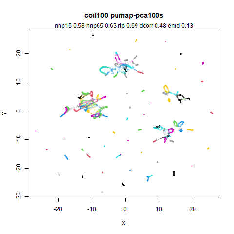 |
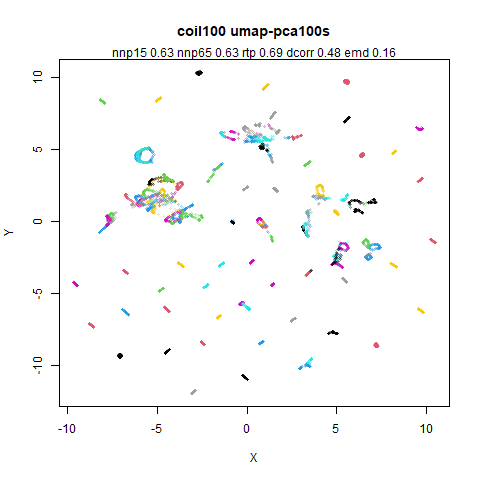
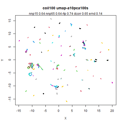
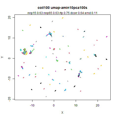
Spectral initialization (perhaps due to lack of a fully connected
graph) seems to affect UMAP’s global metrics, but not the local
preservation. Initializing by PCA makes the rtp and
dcorr metrics similar to PaCMAP.
isofaces
 |
 |
 |
 |
 |
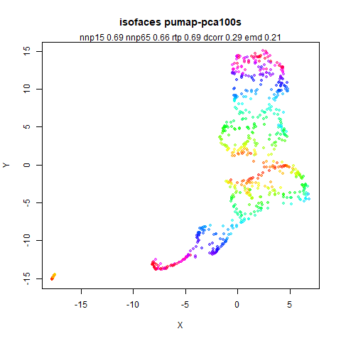 |
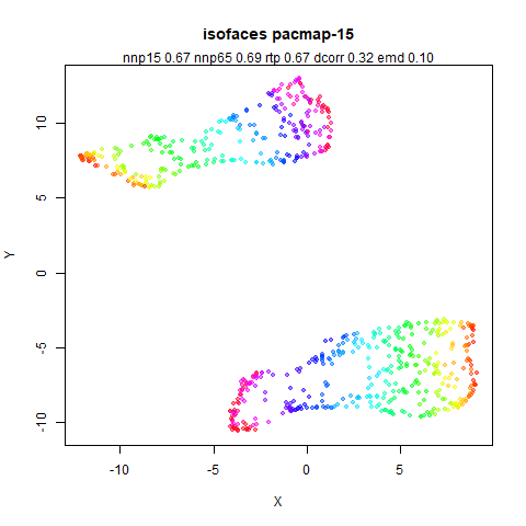
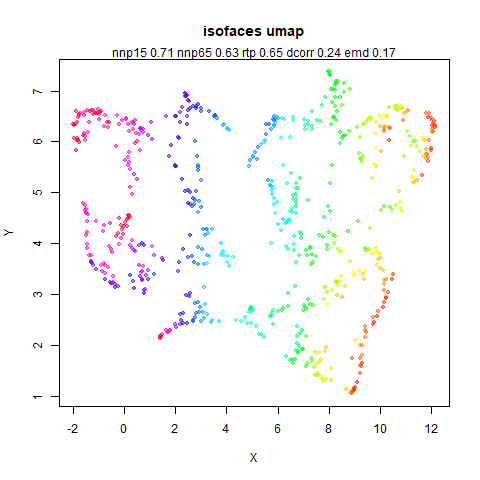
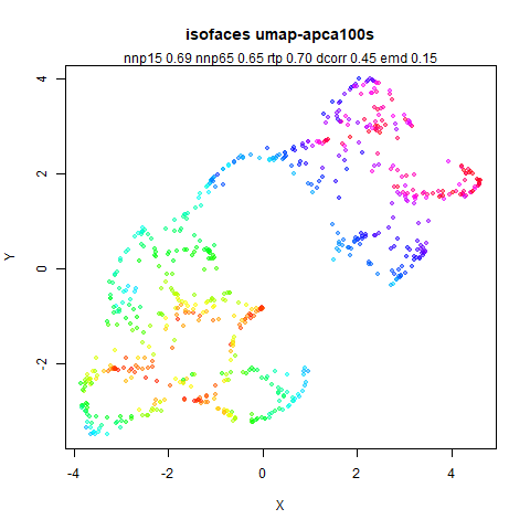
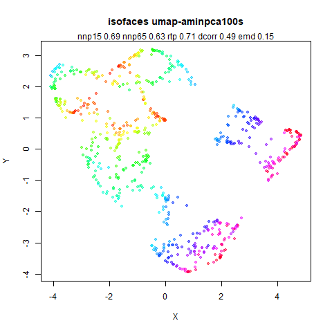
This is not easy to make much sense of. PaCMAP splits the manifold in
two but it still has the best nnp65. dcorr
jumps around a lot, but it doesn’t give a huge amount of guidance to
which of the results is the most visually appealing.
swissroll
 |
 |
 |
 |
 |
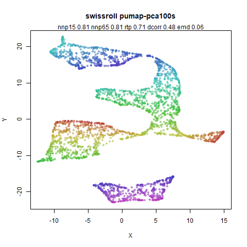 |
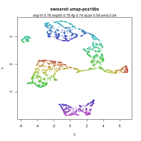
I’ve run PaCMAP a few times and the pictured result is one of its
better results but it always does better than UMAP, which rips the
manifold into lots of little pieces. Adding a PCA-based initialization
cannot be said to help. But you wouldn’t know that from the
dcorr metrics which thinks the PaCMAP result is one of the
worst and the UMAP with Adam (middle right) the best. Interestingly,
while using the PaCMAP forces (bottom right) improves matters greatly,
the basic shape of that result is already in place with UMAP (bottom
left). The difference compared to the middle row results is binarized
edge weights.
At least the local preservation metrics seem to provide a guide here.
Effect of PCA Scaling on Global Metrics
Maybe the problem is that my choice of a “reasonable” PCA scaling
actually isn’t reasonable? Something I noticed when checking what global
metrics looks like for random and PCA-based initializations is that for
some datasets whether the aspect ratio is maintained makes a big
difference with PCA, i.e. scaling the principal components to equal
variance reduces the dcorr and rtp values,
whereas scaling, but keeping the relative ratio of the variance of the
two axes maintains performance. This leads to the question of whether
the axis with the minium or maximum variance should be scaled to the
specified value.
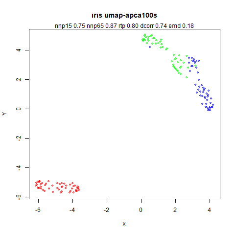
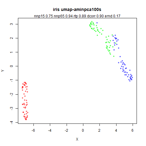
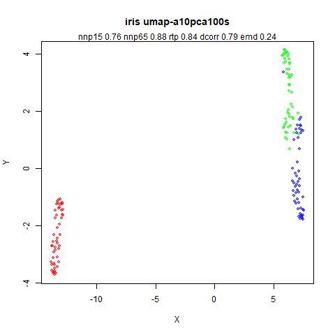
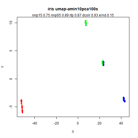
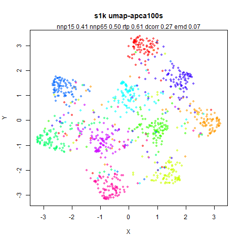
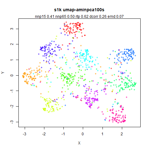
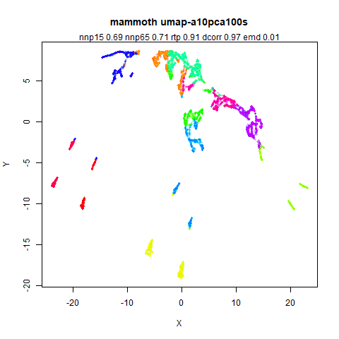
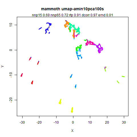
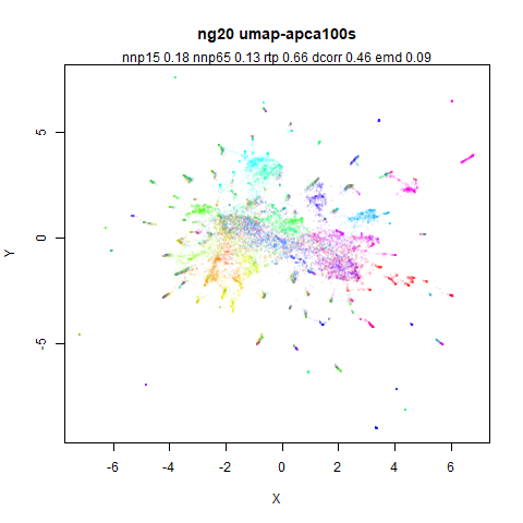
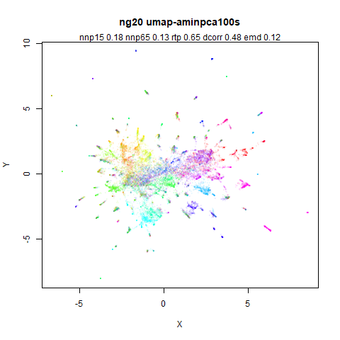
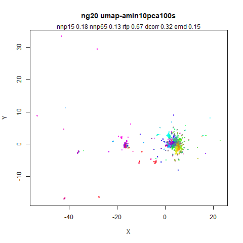
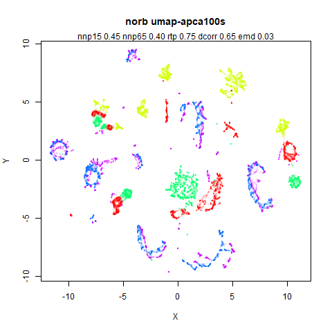
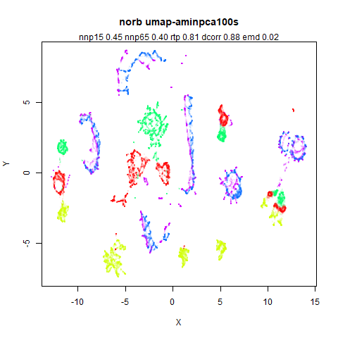
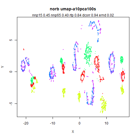
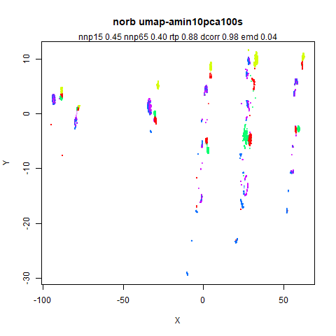
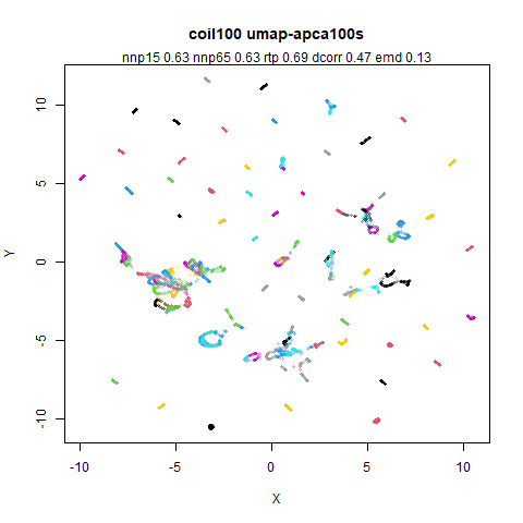
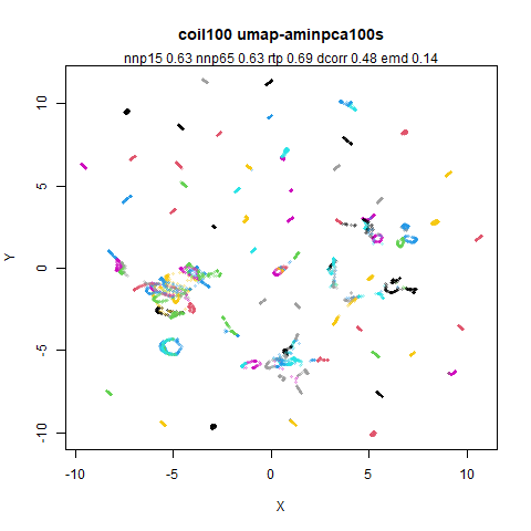
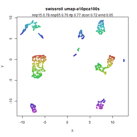
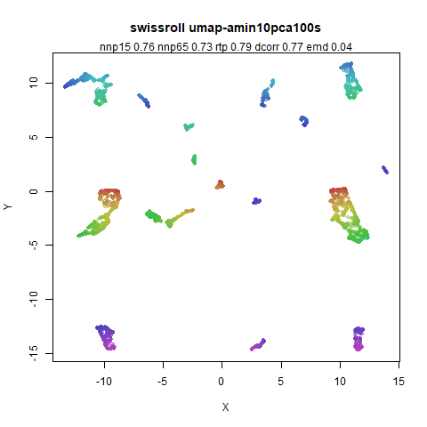
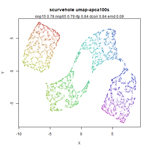
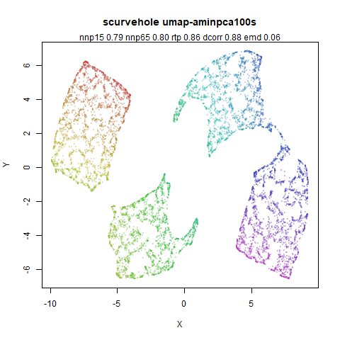
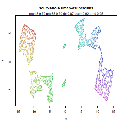
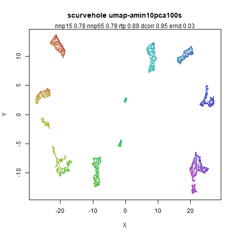
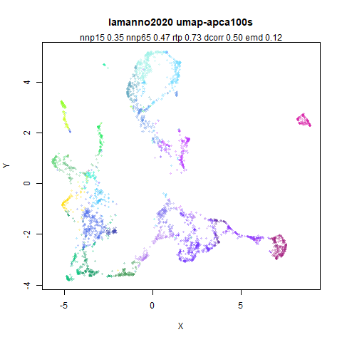
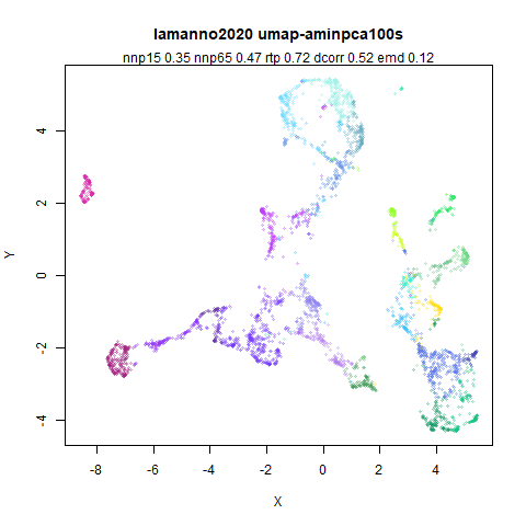
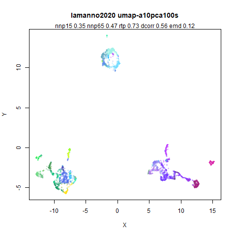
The images below use:
- Top left: Scale the maximum standard deviation dimension to 1.
- Top right: Scale the minimum standard deviation dimension to 1.
- Top left: Scale the maximum standard deviation dimension to 10.
- Top right: Scale the minimum standard deviation dimension to 10.
In all cases, the other dimension is then scaled to keep the standard
deviation proportional to the ratio before scaling. Based on the results
with PCA, I suspect iris and norb to show the
most visual difference in how the initialization is scaled.
dcorr should be more affected than rtp.
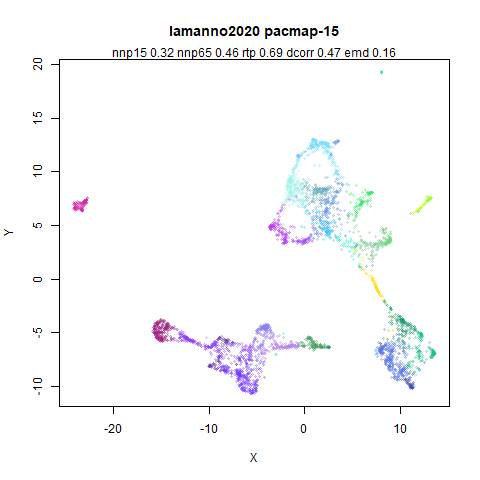
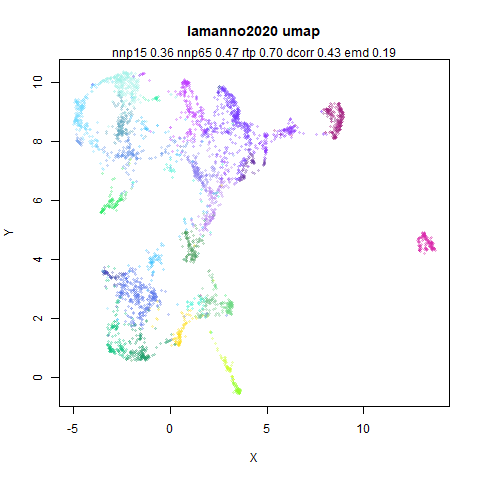
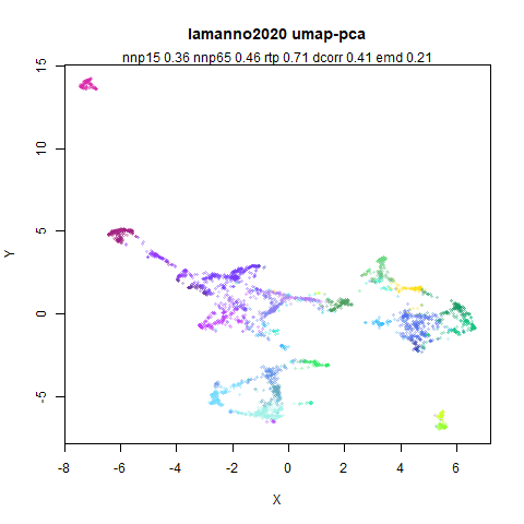
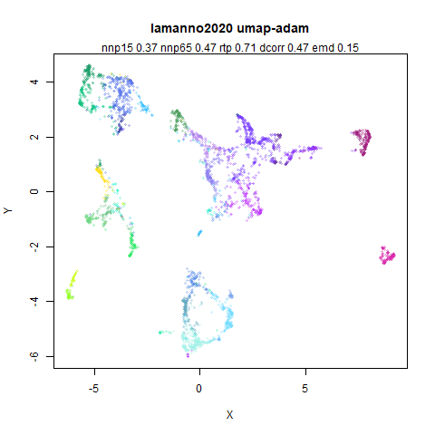
lamanno2020
 |
 |
 |
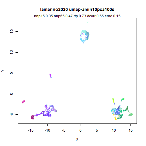 |
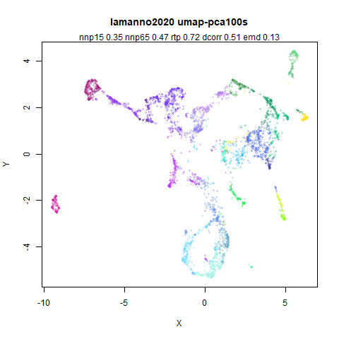
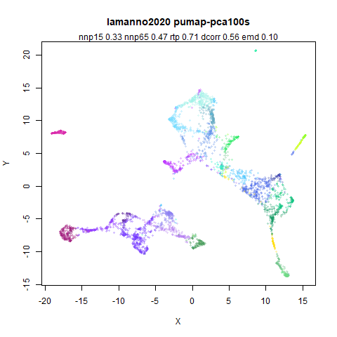
My predictions played out pretty well. Scaling to a standard
deviation of 1, iris and norb aren’t that
different visually, but the dcorr and rtp are
affected.
But it’s with a standard deviation of 10 that things start getting
weird. Visually the output definitely leaves something to be desired.
But the rtp and dcorr values are all really
great. The average rtp and dcorr values all
handily outperform PaCMAP. And in most cases, the local preservation
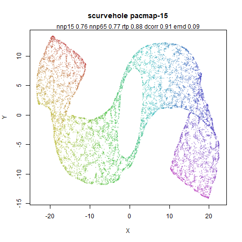
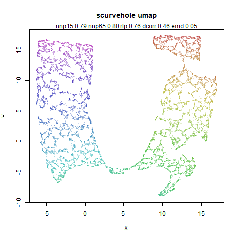
values are the same. frey, swissroll and
scurvehole do show slightly lowered nnp65
values with a standard deviation of 10, but the fall off isn’t as
significant as you might expect given the very different visuals.
Conclusions
Local preservation doesn’t distinguish well between PaCMAP and UMAP. And it does not distinguish well between the very different outputs seen here with UMAP.
For global preservation I still lack a good metric. emd
is cryptic to interpret (at least the way I used it). dcorr
and rtp are also less useful than I had hoped for
preserving global structure, as they can be boosted by increasing the
standard deviation of the initialization leading to some not-very-nice
looking visualizations. rtp seems less sensitive than
dcorr for that at least.
So we are left with the situation that PaCMAP and UMAP produce very simlar looking output. UMAP definitely performs worse for the manifold-like datasets, but these are all quite artificial datasets and their relevance for real-world data is still a question mark for me. On other datasets, the tendency is for UMAP to be a tiny bit better at local preservation, while PaCMAP is better at global preservation. However, what global preservation means here may be a proxy for something like “perturbs the layout that PCA provides as little as possible”. I am not prepared to concede that that is the gold standard measure of global structure at this point (e.g. consider the geodesic distances along the swiss roll vs the ambient distances). However, this may be a worthy and useful goal for large numbers of datasets. And the mid-near pairs may well help with that in PaCMAP, i.e. they are useful even with a well-structure initialization like PCA.
It might also mean that there is a way to sample mid-near pairs in a way that could be easier to integrate into other software: sample them from the PCA output or in fact any other non-random output (e.g. a spectral layout). This could retain more of that initial structure while only requiring calculating Euclidean distances from the output data, which is already something that UMAP and related codebases do. This is a much easier task than having to replicate the different distance metrics available in nearest neighbor libraries. Also, the actual input data may not be present: you could provide a pre-computed nearest neighbor graph as input. PCA can’t be carried out on that, but a spectral initialization on the input graph is still possible.