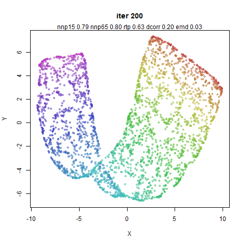
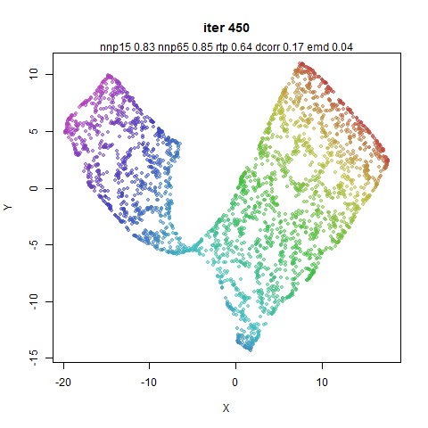
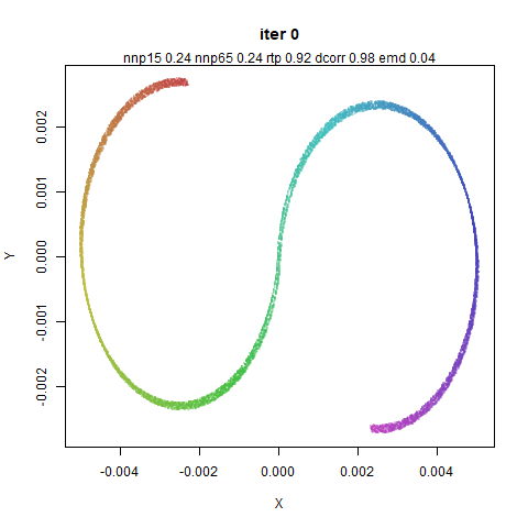
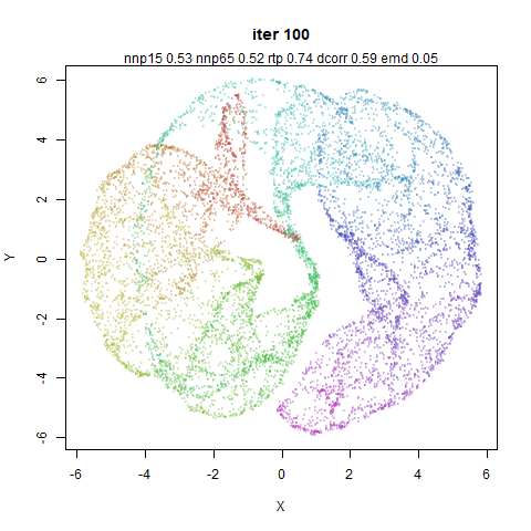
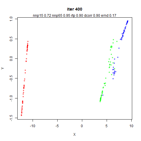
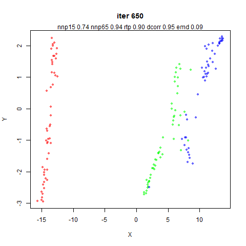
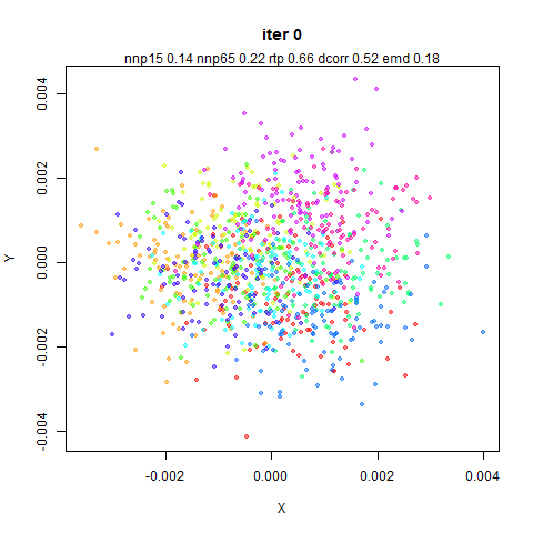
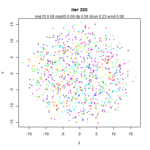
Way Too Many Images of PaCMAP Embeddings
Brace yourselves. What follows are some snapshots of quite a large
number of datasets as PaCMAP embeds them (there are lots of these in the
PaCMAP paper too). I have then gone and manipulated the Python source
code to attempt to satisfy my curiosity about which things are most
important.
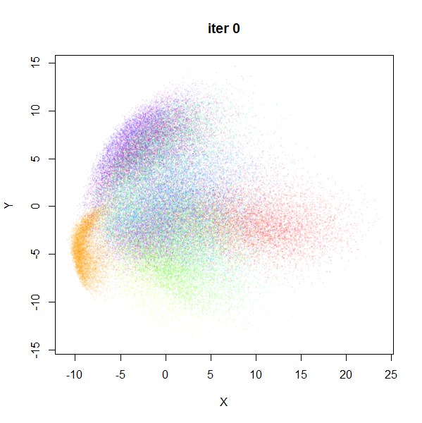
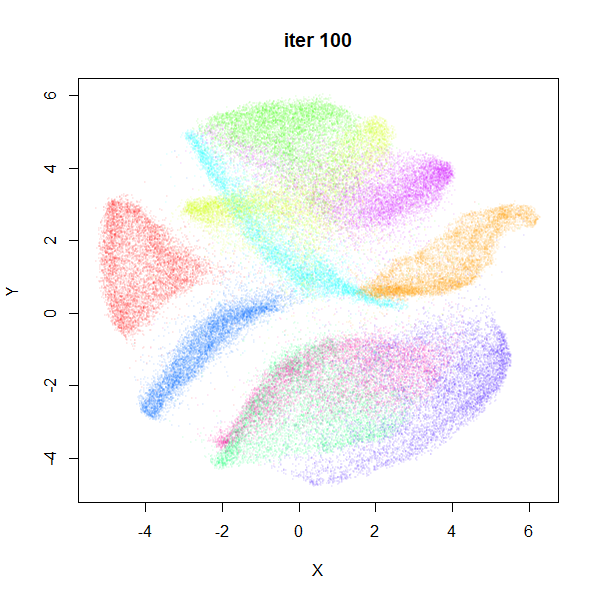
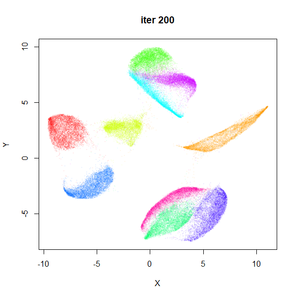
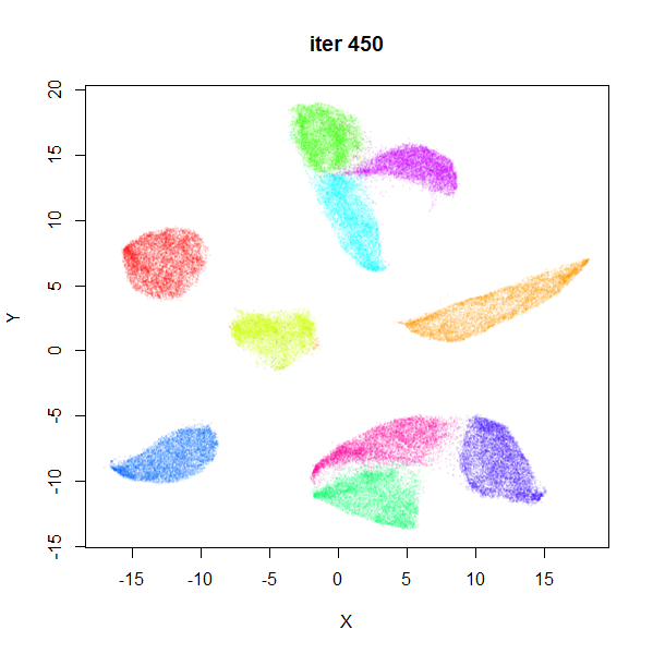
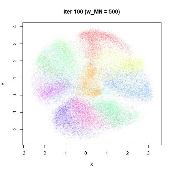
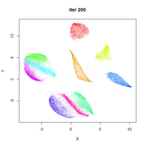
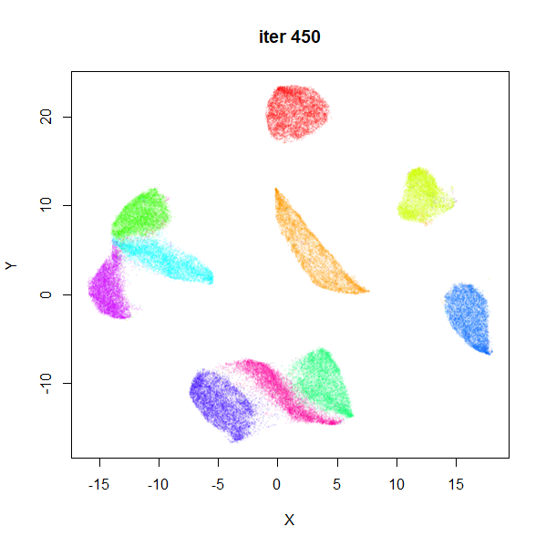
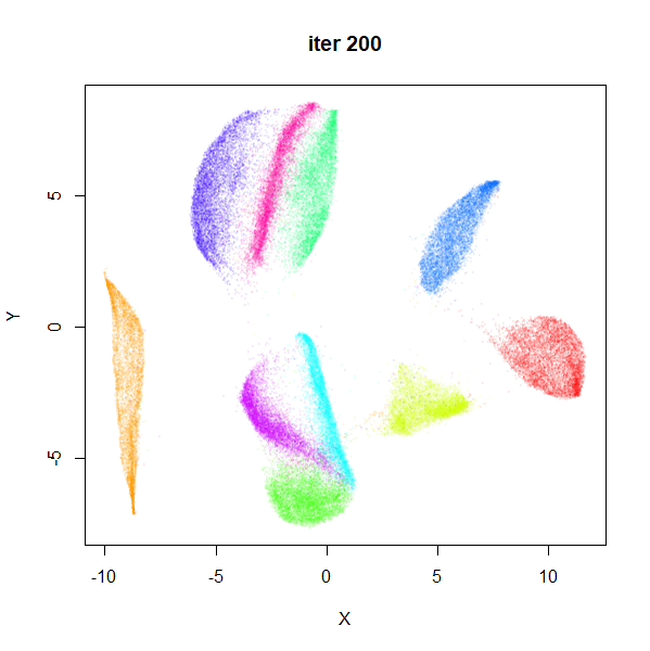
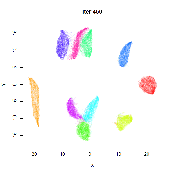
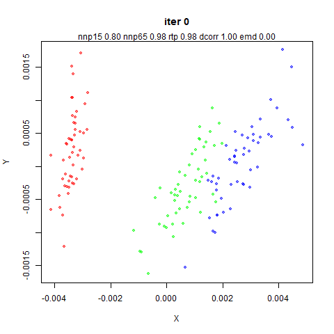
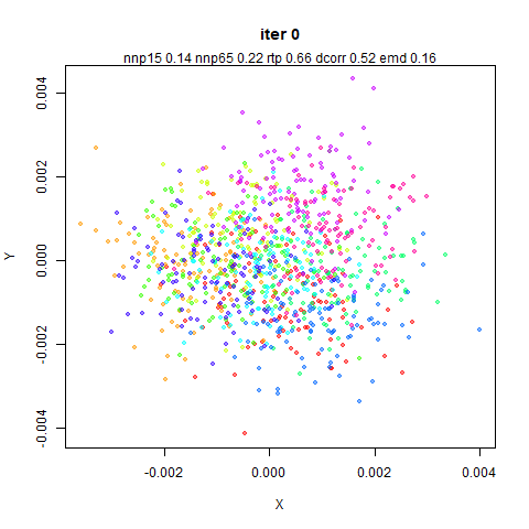
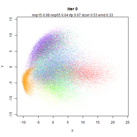
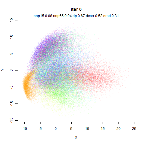
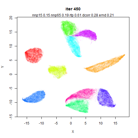
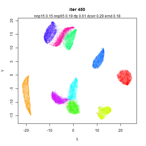
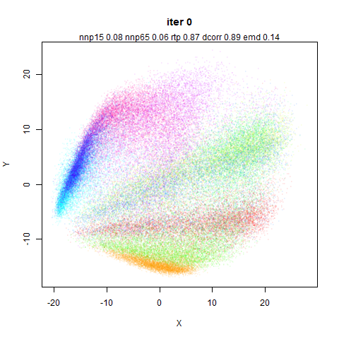
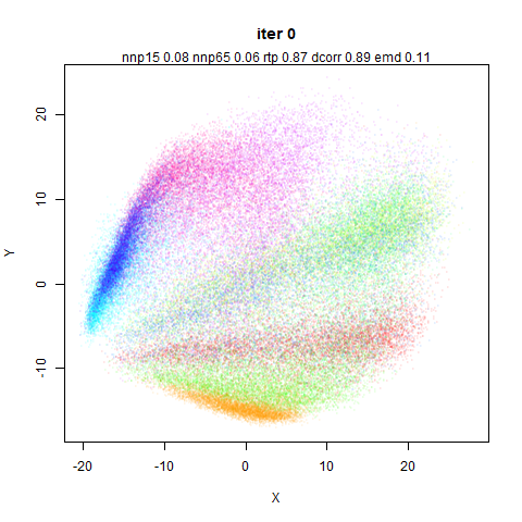
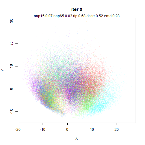
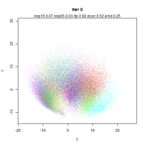
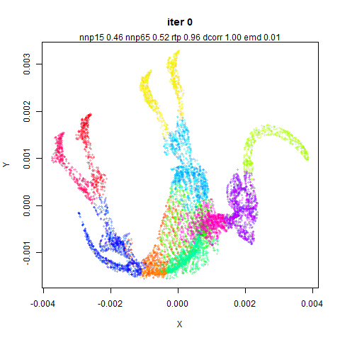
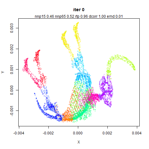
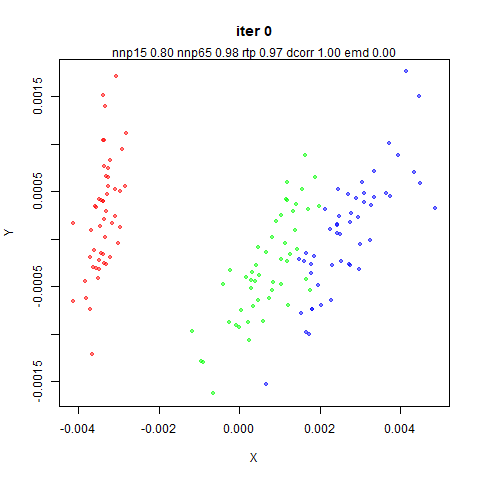
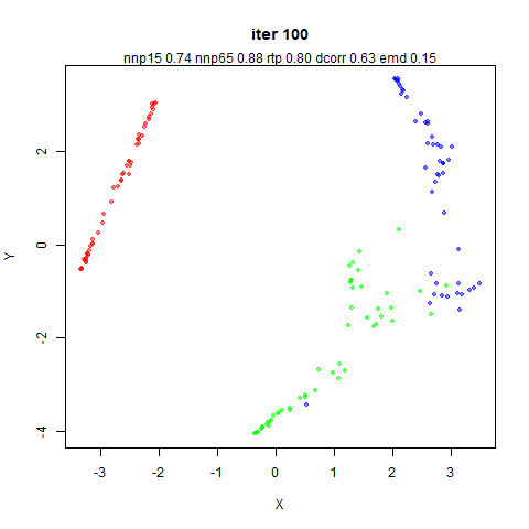
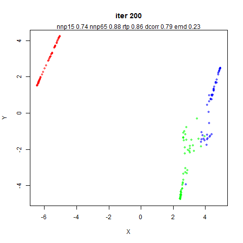
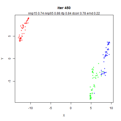
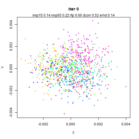
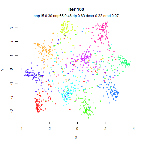
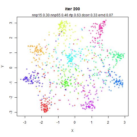
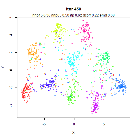
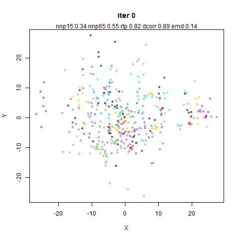
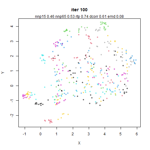
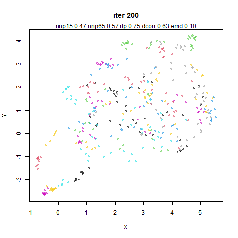
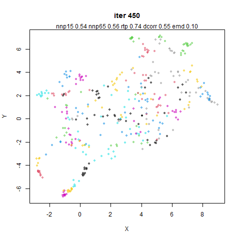
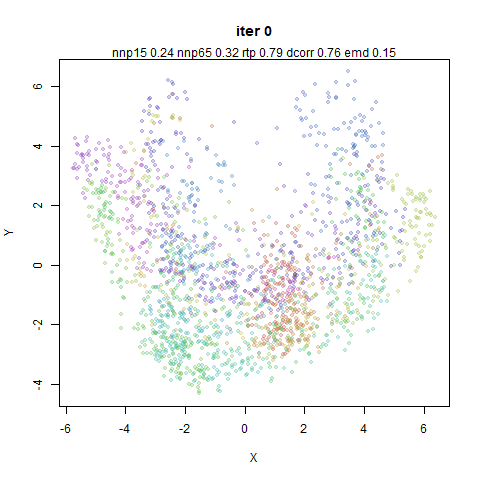
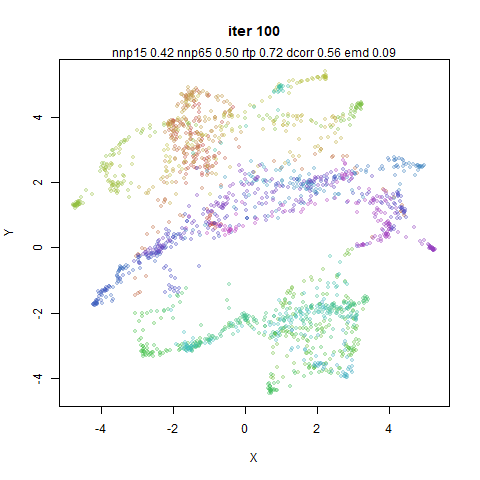
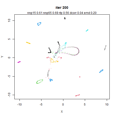
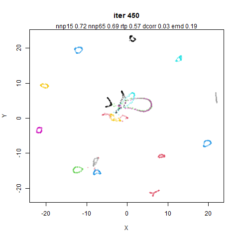
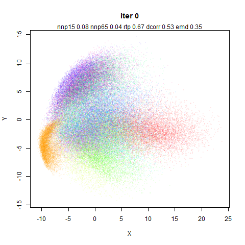
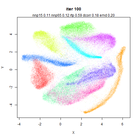
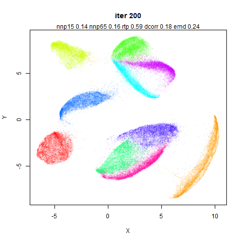
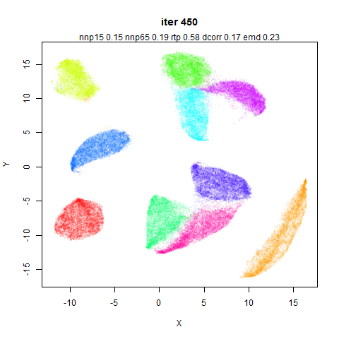
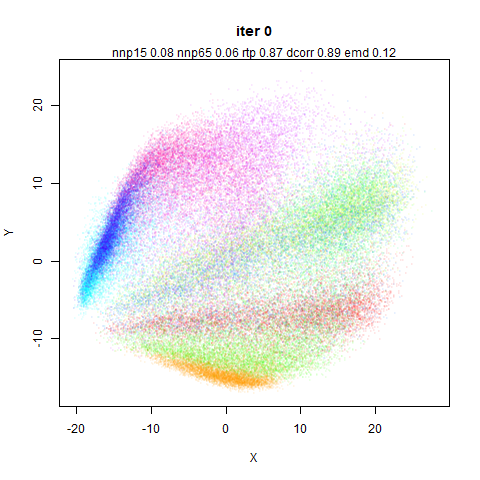
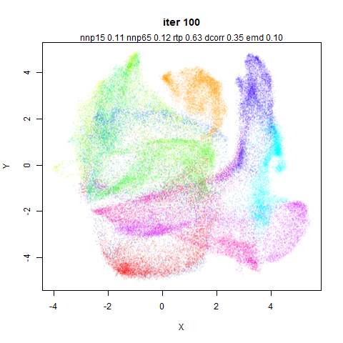
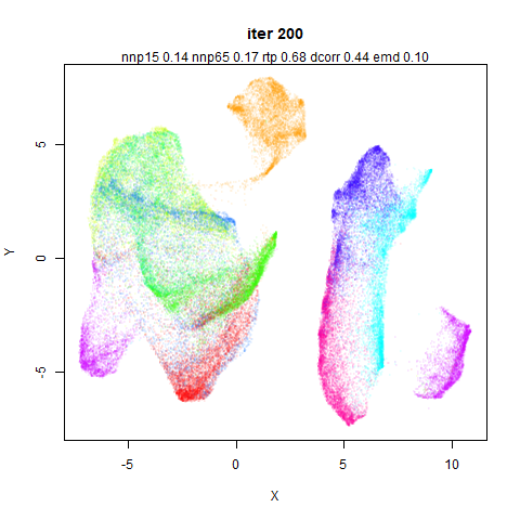
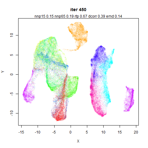
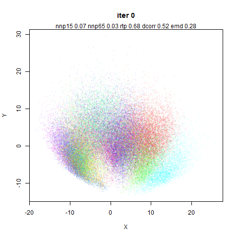
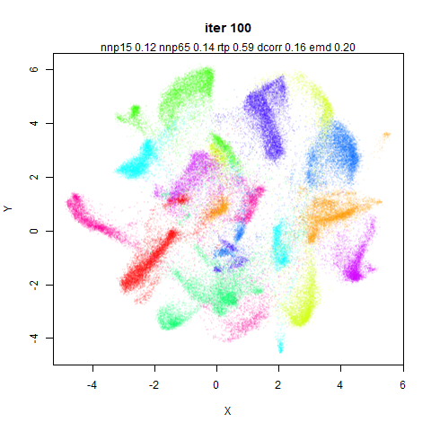
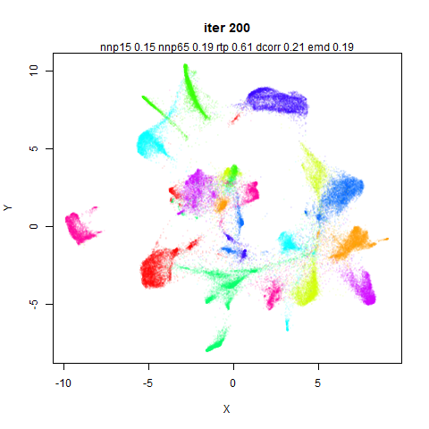
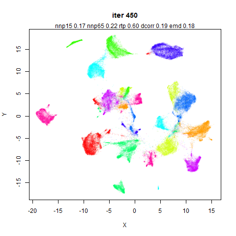
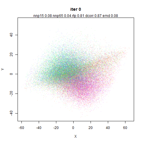
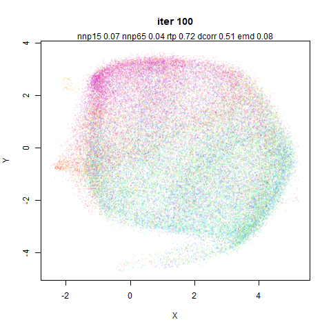
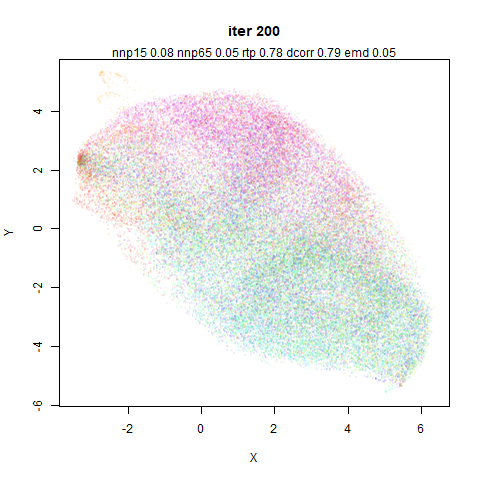
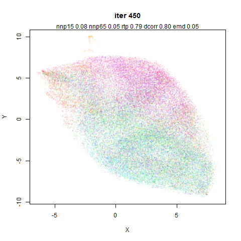
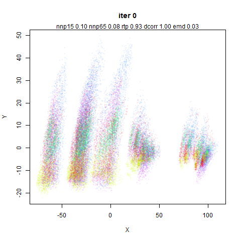
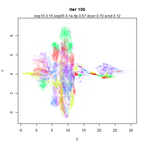
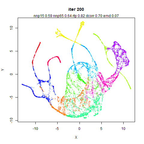
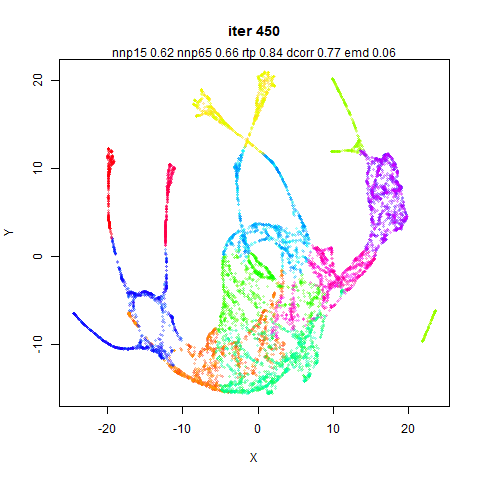
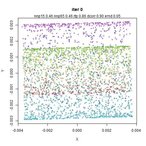
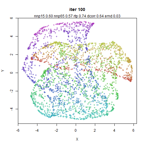
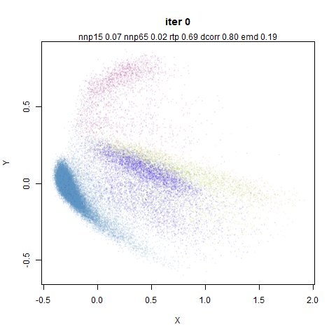
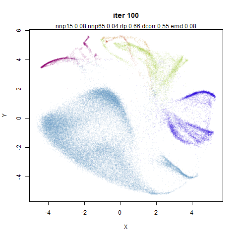
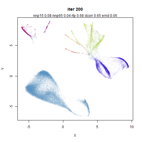
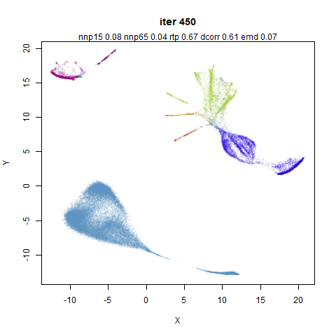
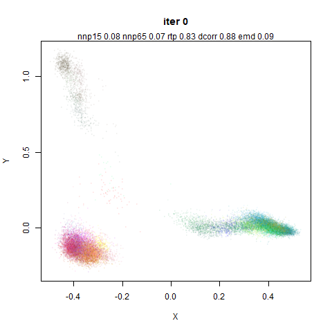
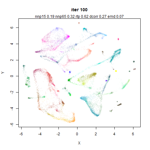
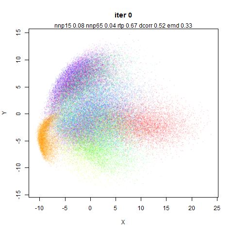
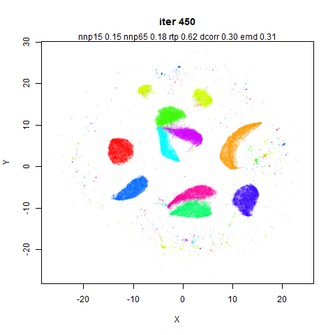
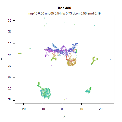
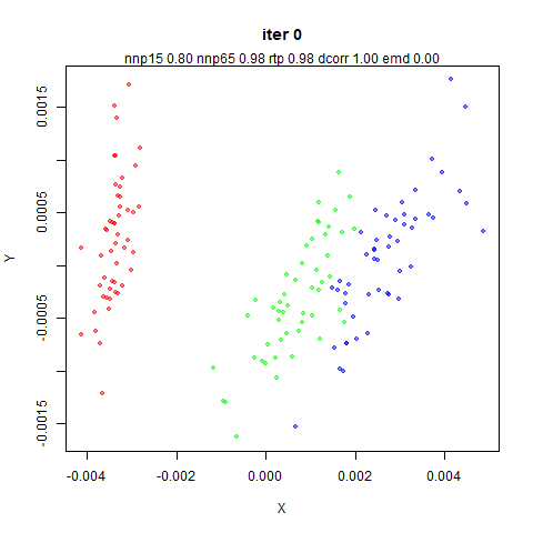
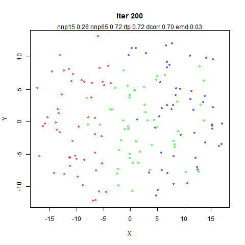
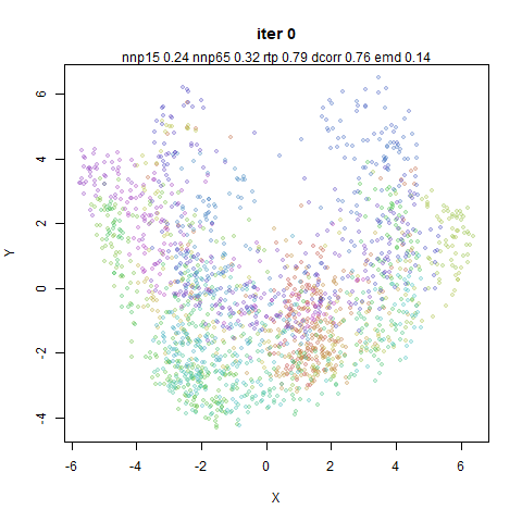
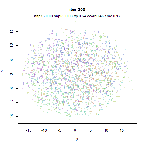
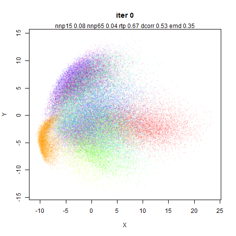
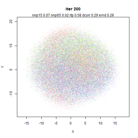
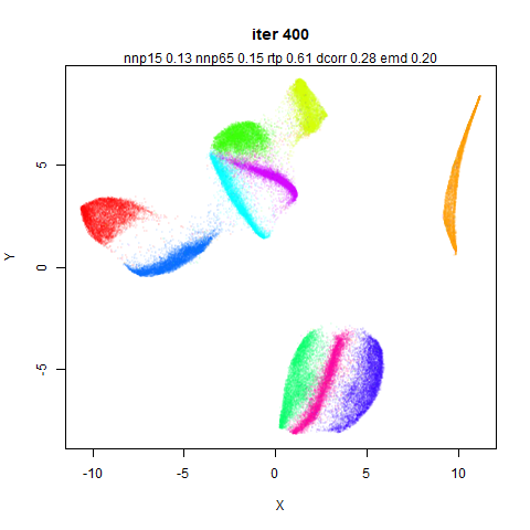
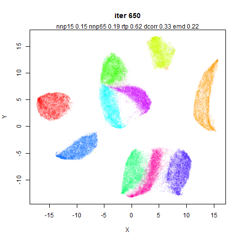
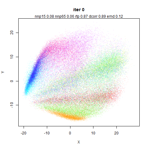
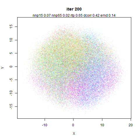
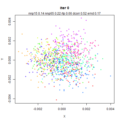
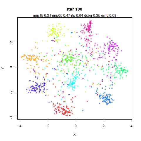
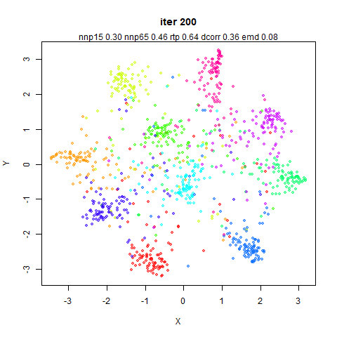
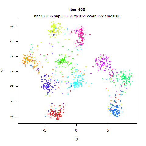
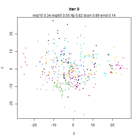
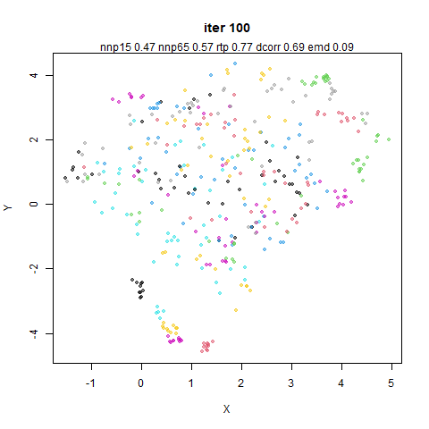
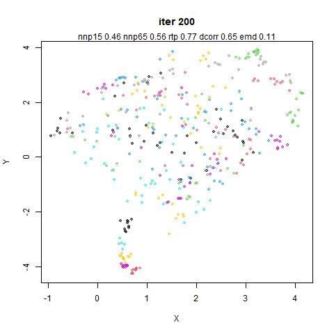
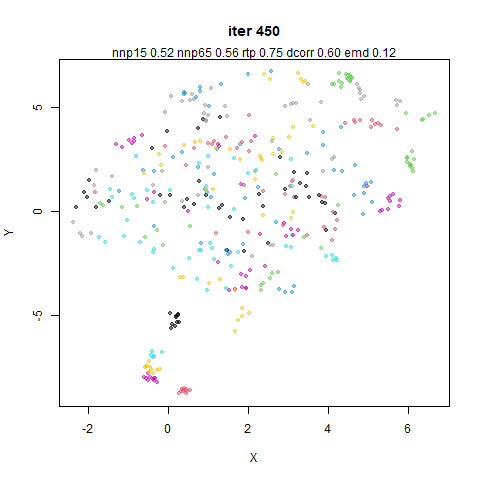
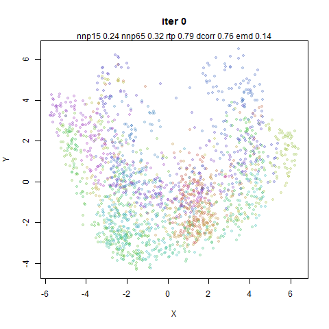
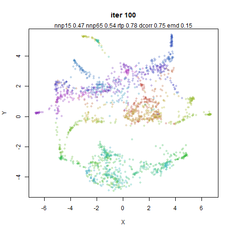
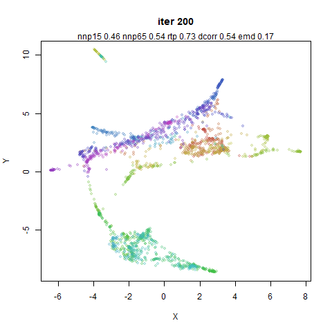
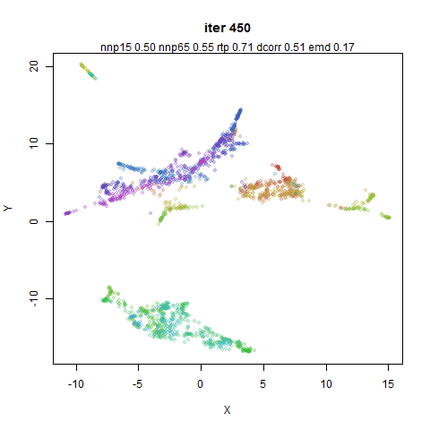
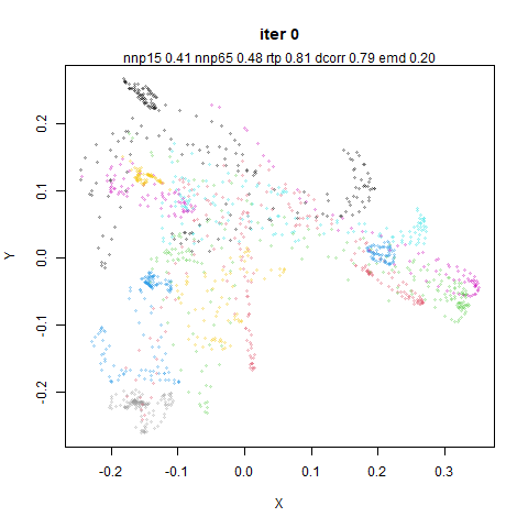
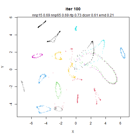
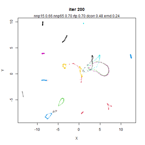
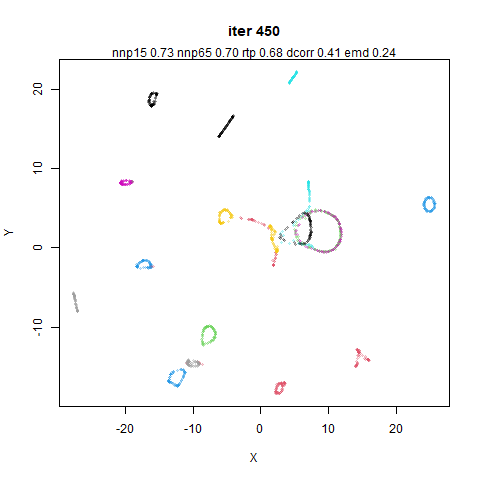
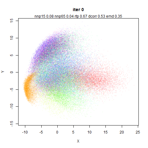
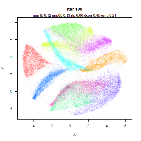
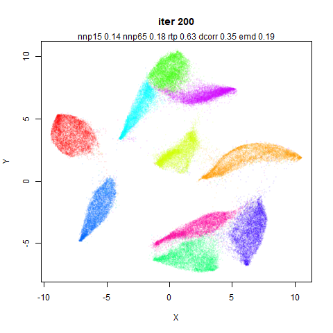
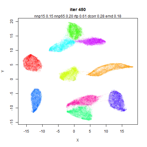
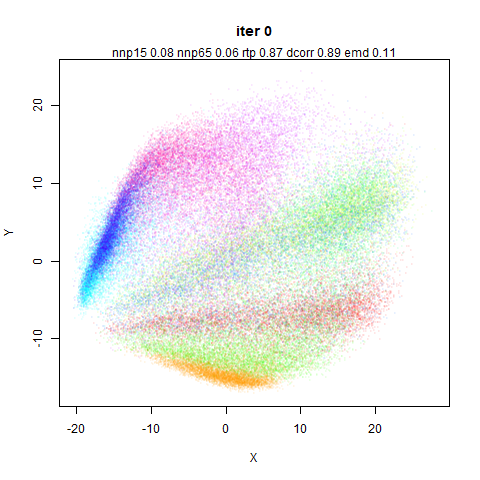
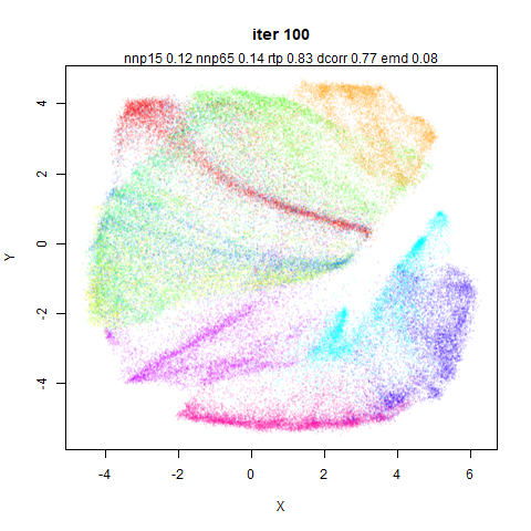
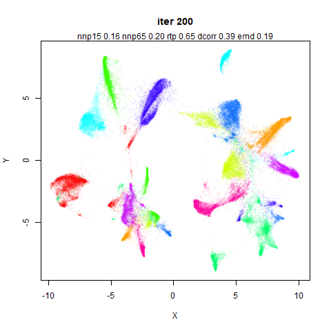
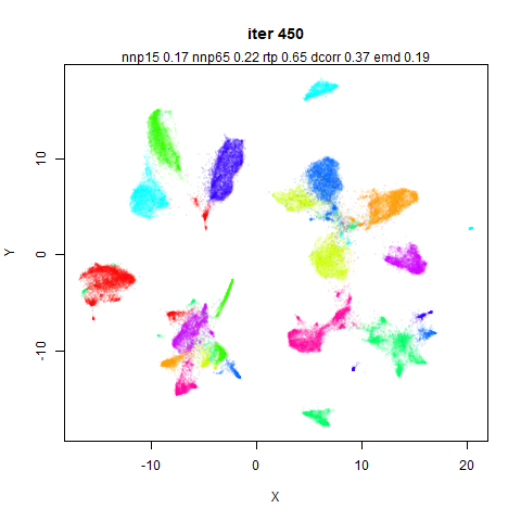
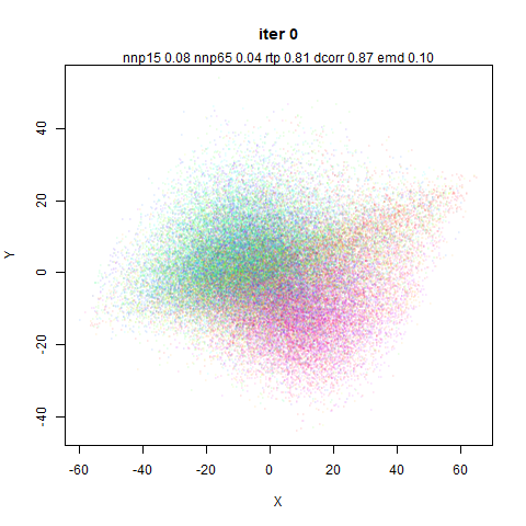
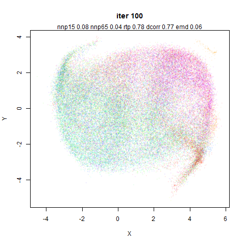
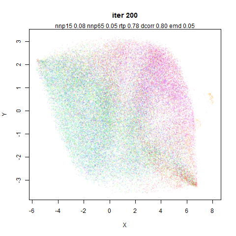
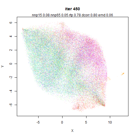
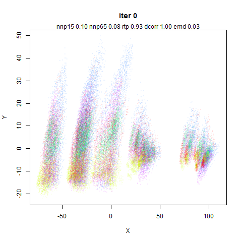
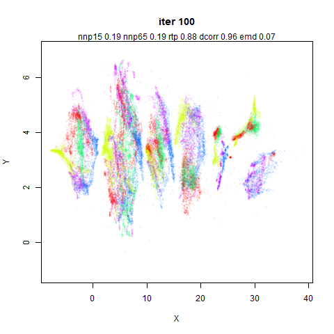
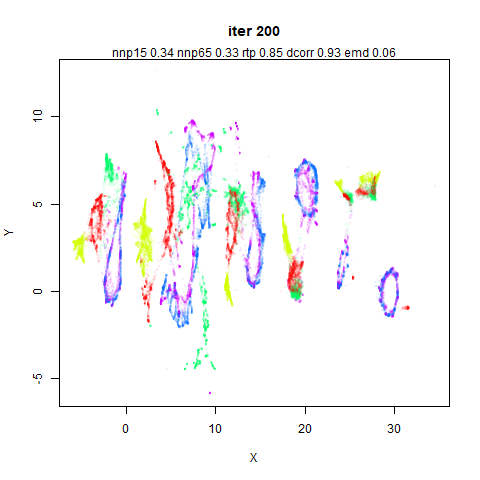
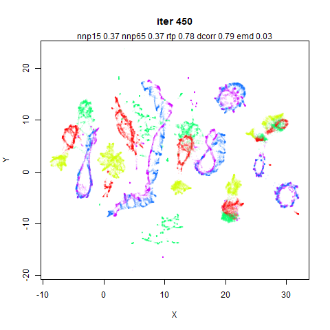
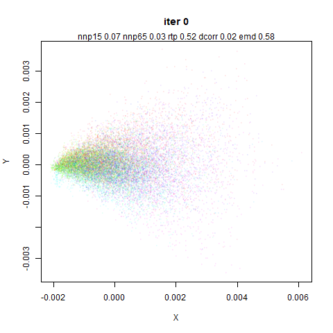
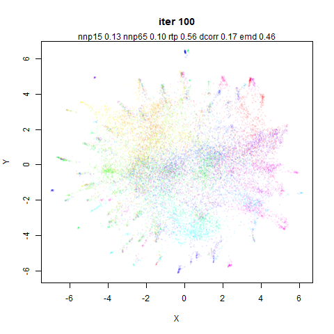
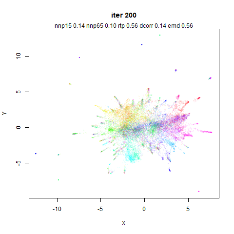
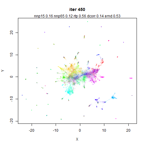
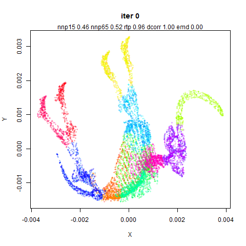
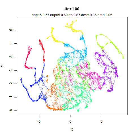
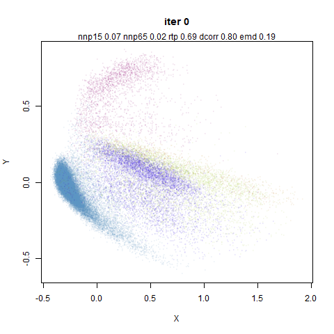
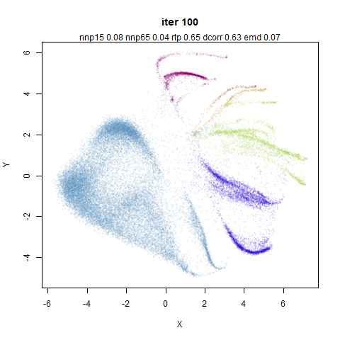
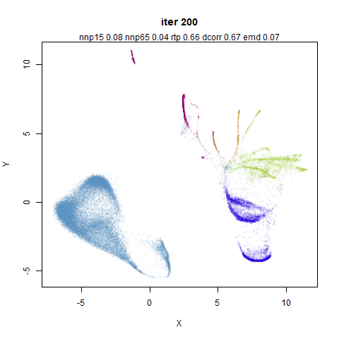
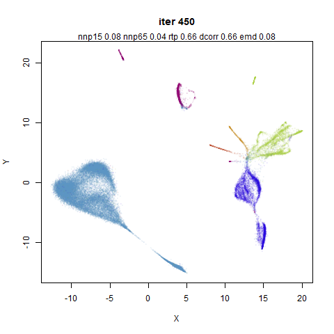
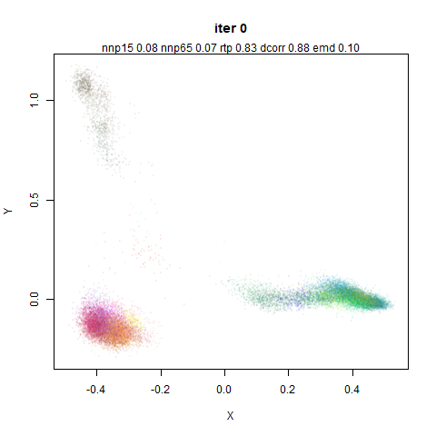
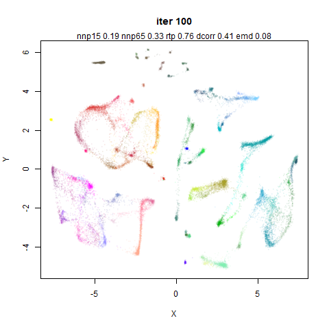
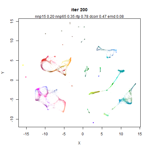
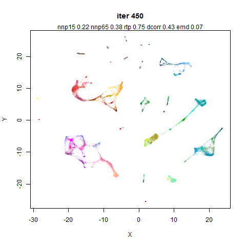
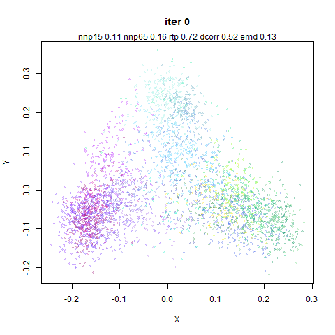
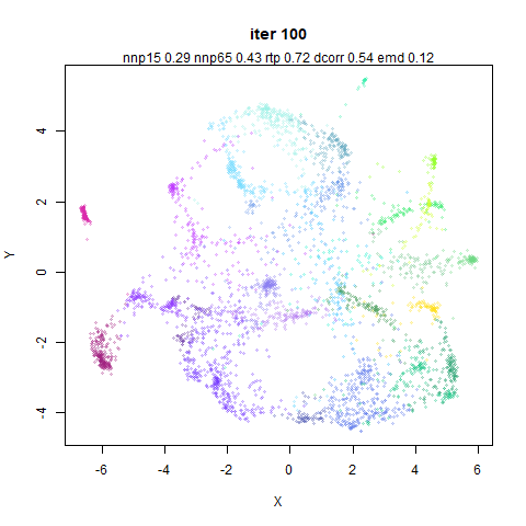
Let’s start nice and easy. Here’s four images of MNIST at the
following iterations: top left 0, top right 100 (at the end of the first
phase of optimization), bottom left 200 (at the end of the second phase
where mid-near forces are turned off) and bottom right 450 iterations
(final output).
The influence of the mid-near neighbors by iteration 100 is clear in
the form of the expanded clusters. It can also be seen that subsequent
iterations don’t do much to the basic structure of the embedding, but
rather refine and separate any existing clusters. However, it’s
interesting that there is some indication of clustering at iteration 0
(the PCA input) but it is not reflected at iteration 100. This
is most easily seen with the orange cluster (those are the ‘1’ digits),
which is on the left hand side at iteration 0, but has moved to the
right hand side at iteration 100. These coordinates are directly output
from PaCMAP without any other transformation so it genuinely has moved.
Almost certainly this is due to the very large initial mid-pair forces.
Whether this is a good thing probably depends on whether you think the
basic structure of the PCA initialization should be preserved or
not.
To demonstrate the influence of the mid-near weights initially, here
is the same embedding but instead of linearly ramping the weight down
from 1000 to 3 over the first 100 iterations, we fix w_{\mathrm{MN}}=500 (basically the average
over the linear ramp):
The 1 cluster is now only moved into the center of the plot. The
final shape of the clusters remains the same, but their relative
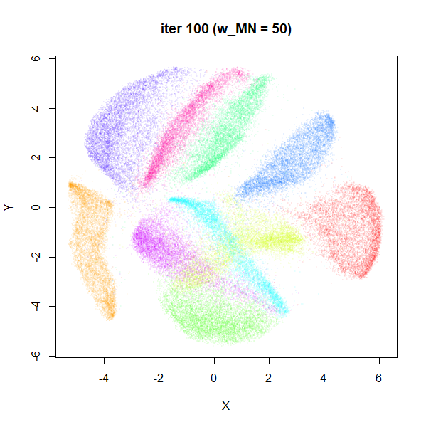
position and orientation has changed. If we drop the mid-near weights an
order of magnitude to w_{\mathrm{MN}}=50 (still itself an order of
magnitude higher than the near pair weight) we can make the 1 cluster
stay close to its location in the initial coordinates:
Once again the clusters have familiar shape but a new
arrangement.
Three different weight schemes to the mid-near points, and three
different global outcomes. Which is best? Here’s a table with some
measures of distortion, compared to the raw input data (i.e. no scaling
or PCA applied).
| linear |
0.15 |
0.19 |
0.61 |
0.29 |
0.22 |
| 500 |
0.15 |
0.19 |
0.64 |
0.41 |
0.21 |
| 50 |
0.15 |
0.19 |
0.62 |
0.32 |
0.22 |
np15 and np65 measure the preservation of
the 15 and 65 nearest neighbors respectively. triplet
measures the random triplet accuracy (as used in the PaCMAP paper) with
20 triplets per point. Pearson measures the Pearson correlation between
100,000 randomly chosen pairs of points in the input and output space
(similar to the method uses by Becht and co-workers).
EMD is the Earth Mover’s Distance method similar to that
used by Heiser
and Lau.
In terms of local neighborhood preservation, there is no difference.
Of the global measures, neither the triplet preservation nor EMD
indicate show a big difference either. The Pearson correlation shows a
bigger change, favoring the w_{\mathrm{MN}}=500 approach. For what it’s
worth, it does also show the best triplet preservation and the
smallest EMD, but I don’t know if the size of the differences really
mean anything.
Turning Off Mid Pair Forces
PaCMAP’s ability to focus on global structure depends strongly on the
mid-near pairs to differentiate itself from something like UMAP. What
happens if we turn it off? Probably not much. The paper itself stresses
that a PCA-style initialization gives good results, and the mid-near
pairs are what is useful for retaining global structure with random or
other less-structured initialization.
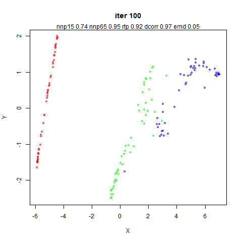
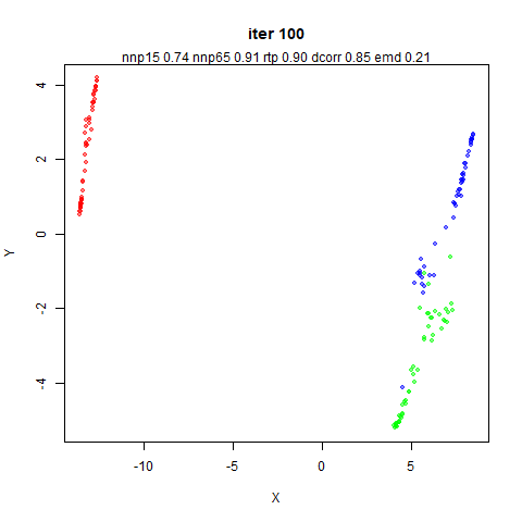
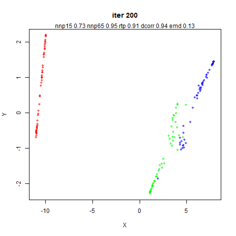
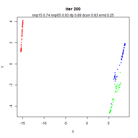
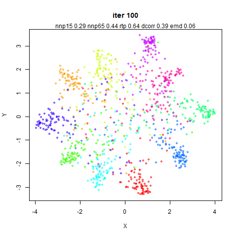
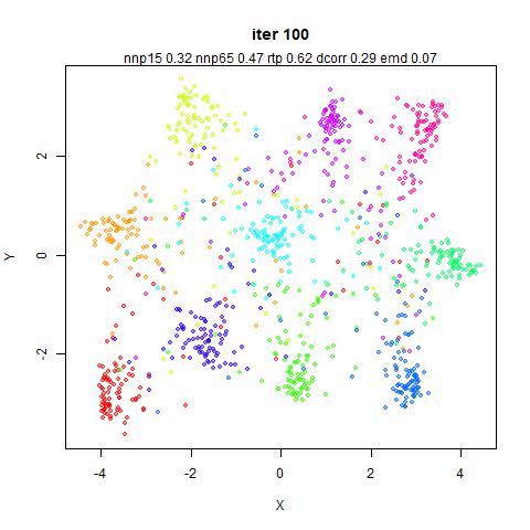
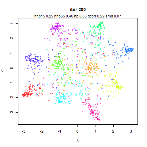
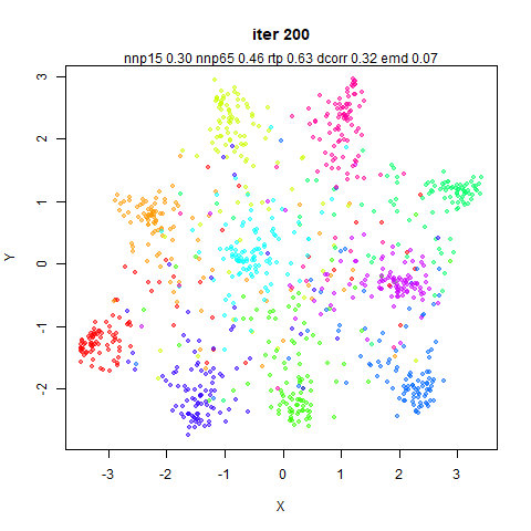
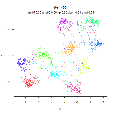
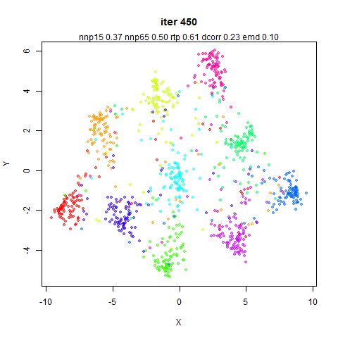
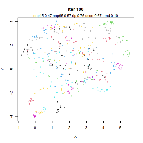
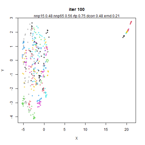
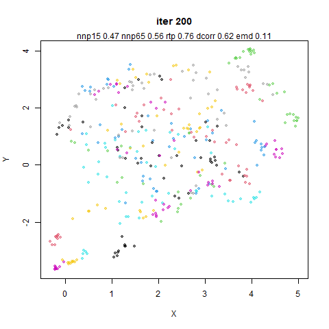
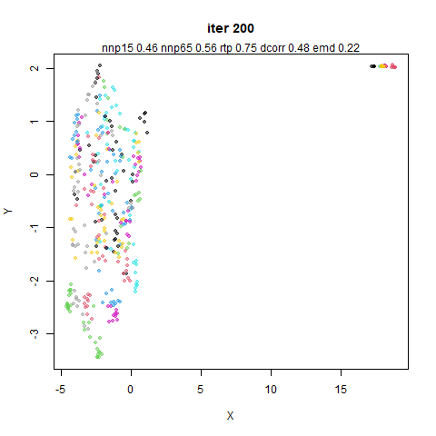
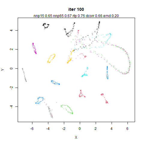
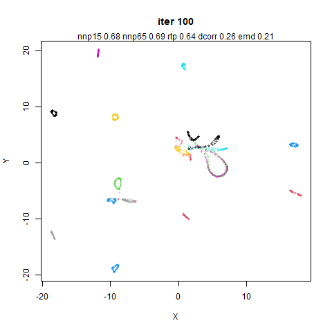
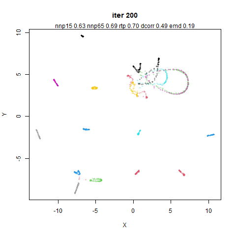
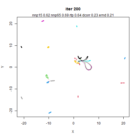
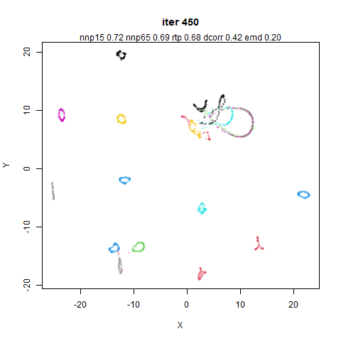
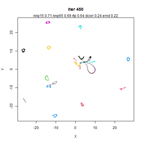
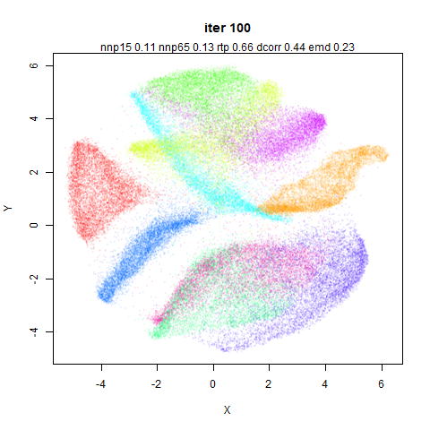
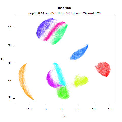
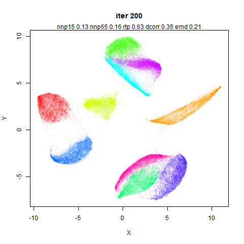
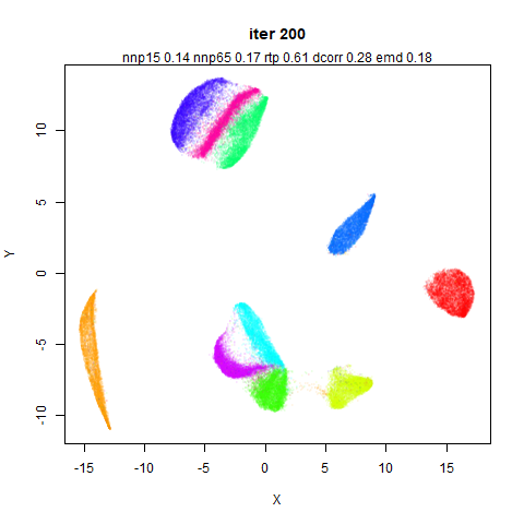
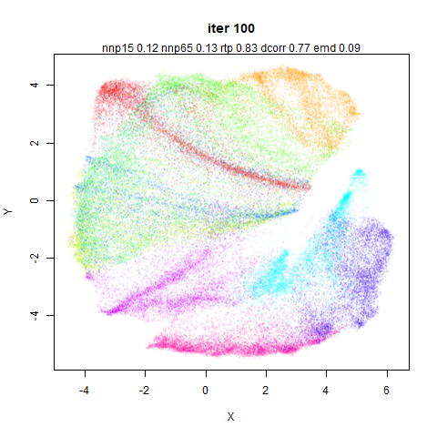
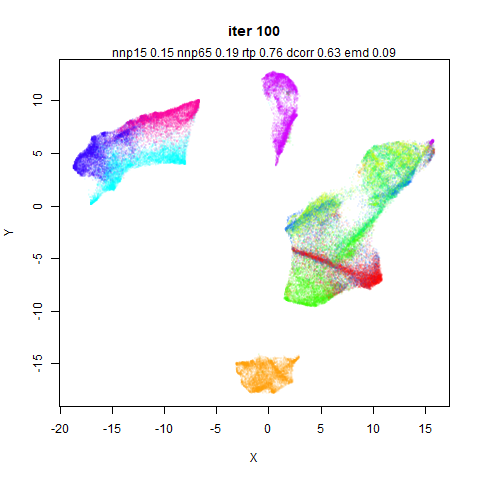
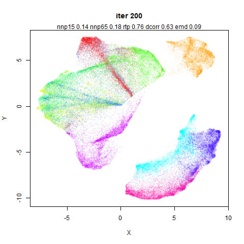
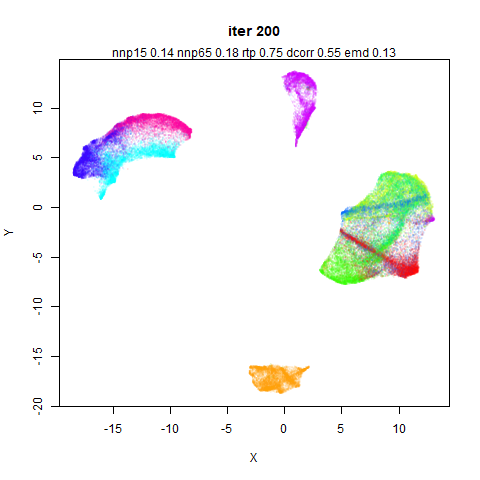
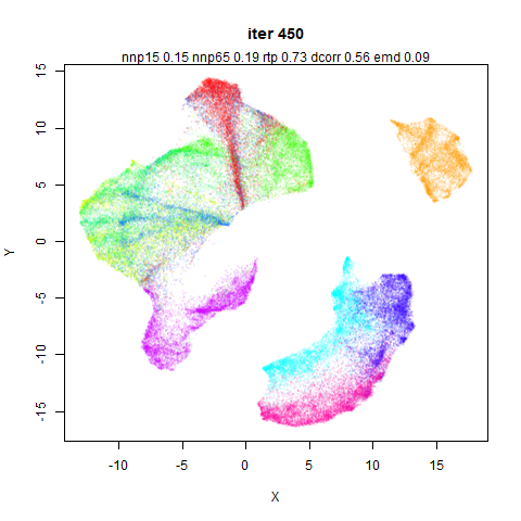
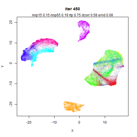
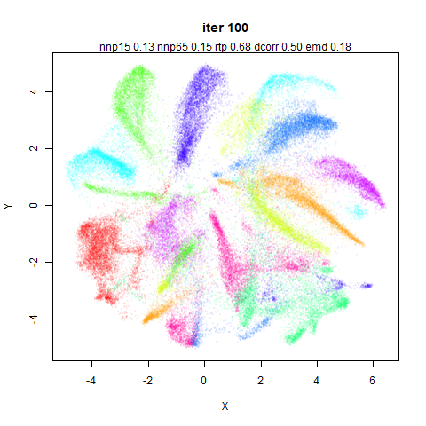
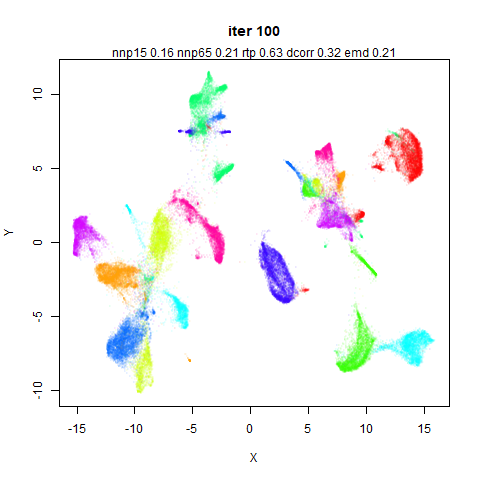
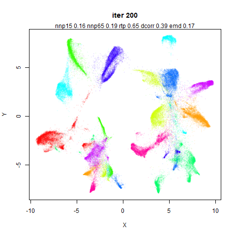
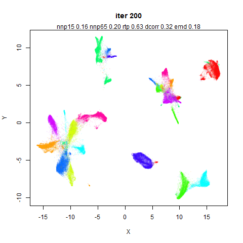
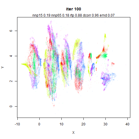
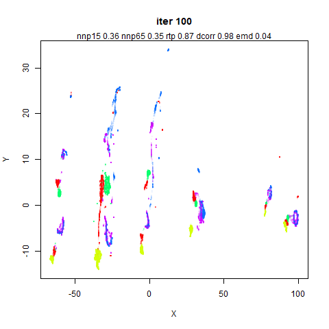
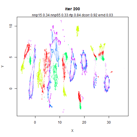
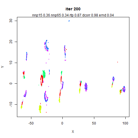
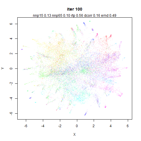
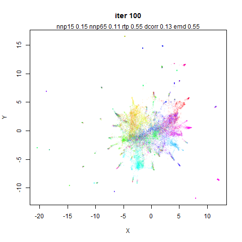
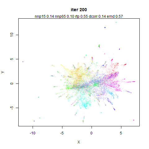
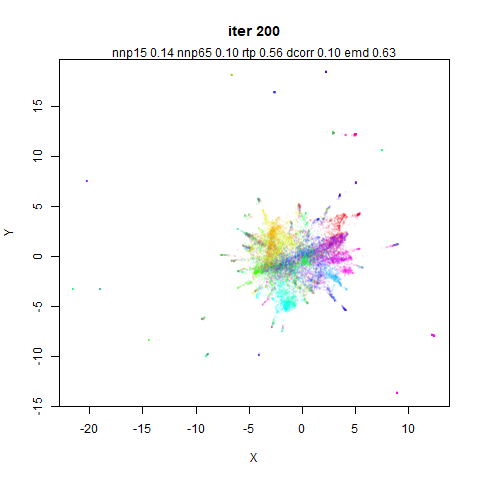
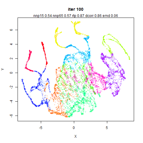
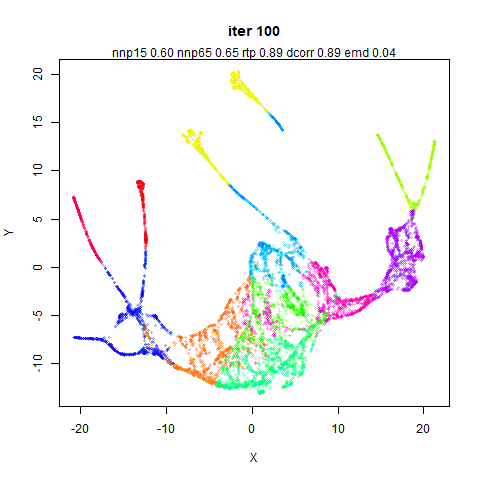
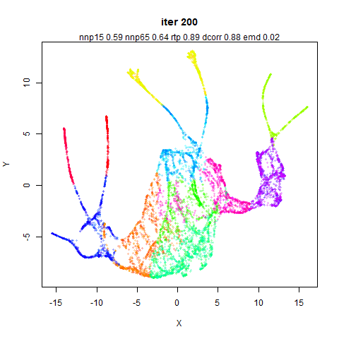
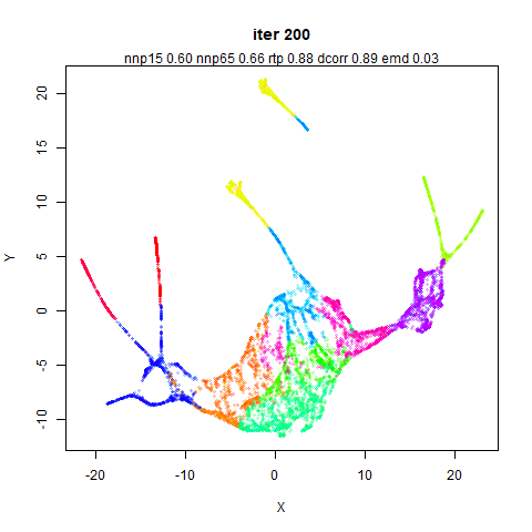
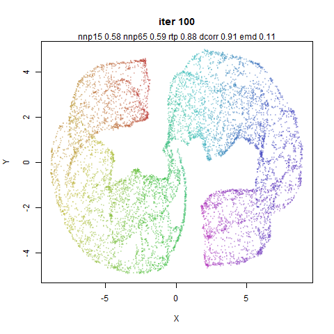
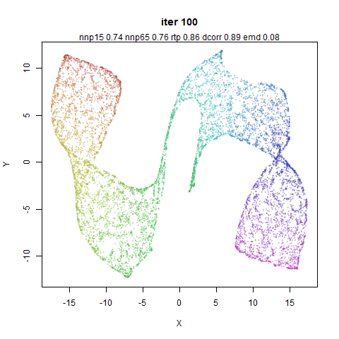
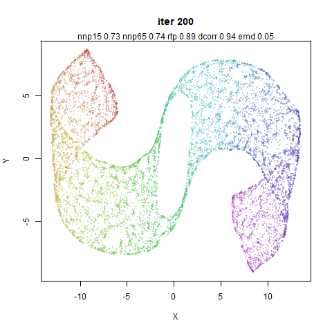
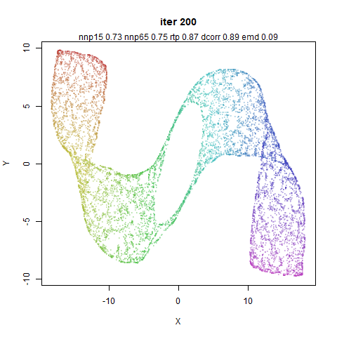
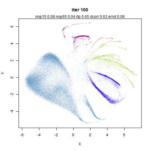
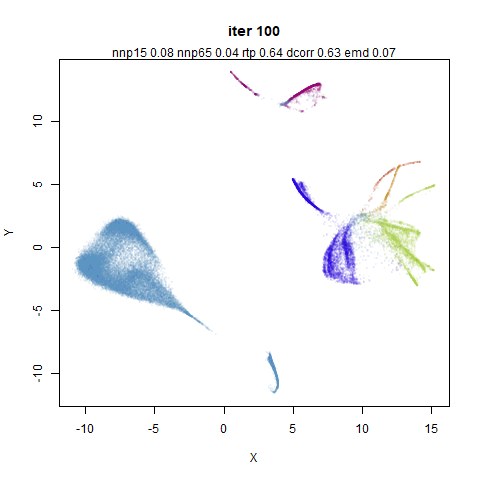
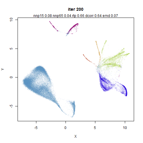
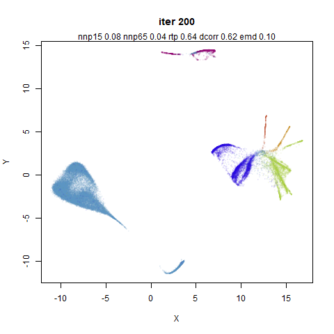
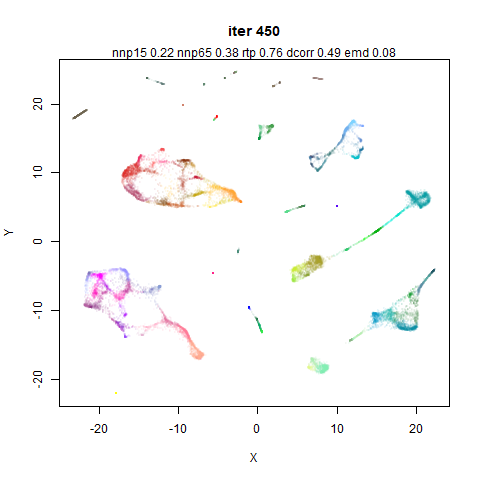
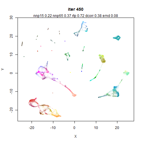
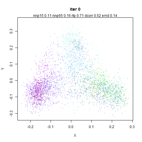
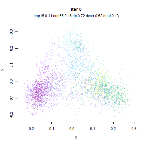
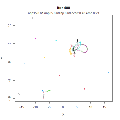
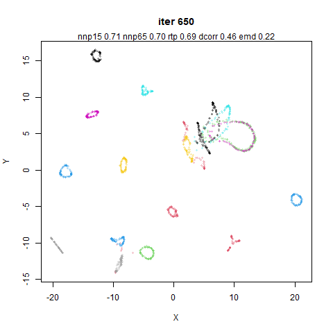
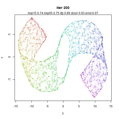
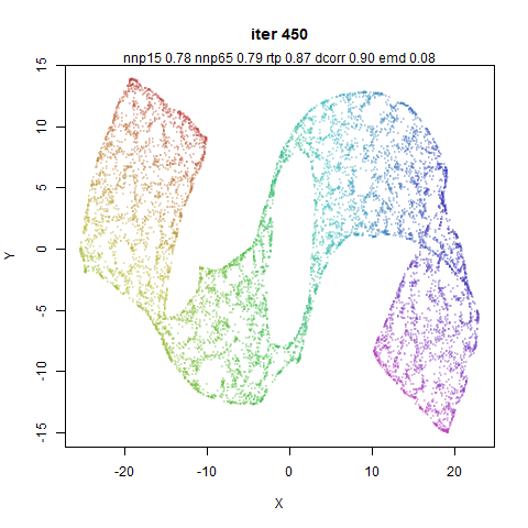
Anyway, let’s find out. In the images below, each column is a
different run, and each row is a different iteration number, so you read
down the column to see how a given optimization plays out. The left-hand
column is PaCMAP with default settings except the the number of
neighbors is fixed to 15, i.e. n_neighbors=15. The right
hand column is the same except I have set the mid-near weights to always
be 0. Arguably, I could/should set the near-pair weights to always be 1,
but I didn’t want to change too much at once. Presumably the last 250
iterations can recover from any over-attraction.
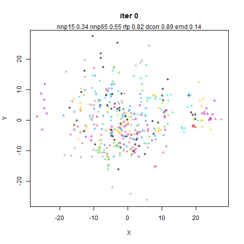
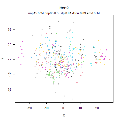
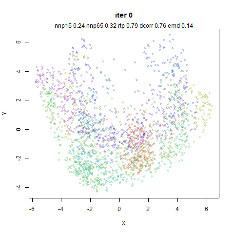
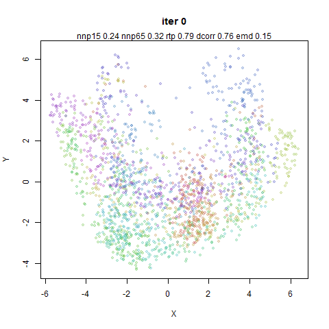
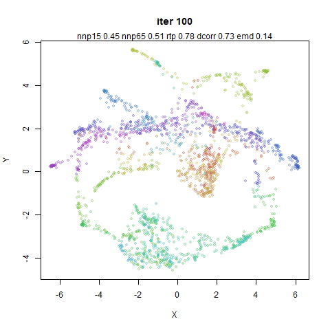
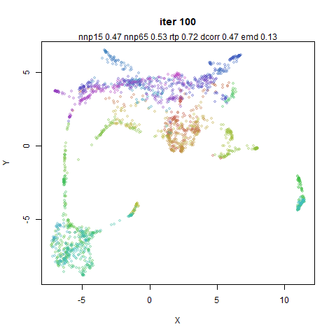
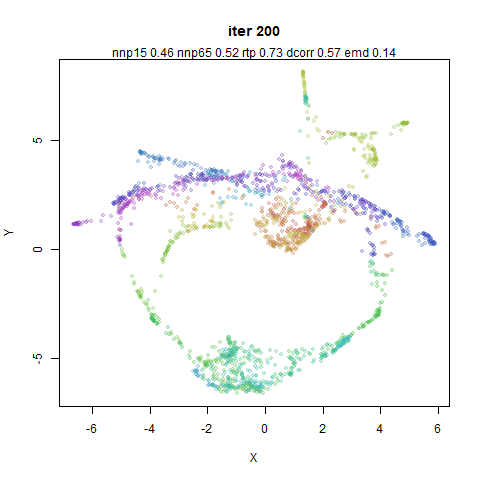
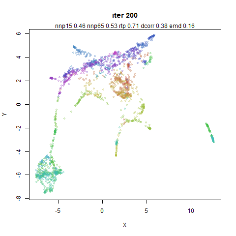
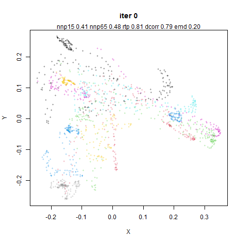
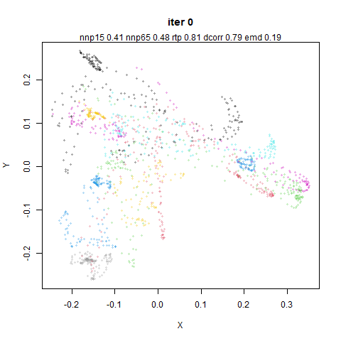
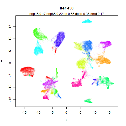
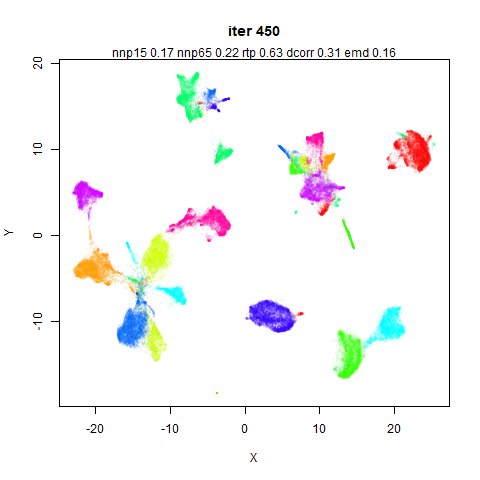
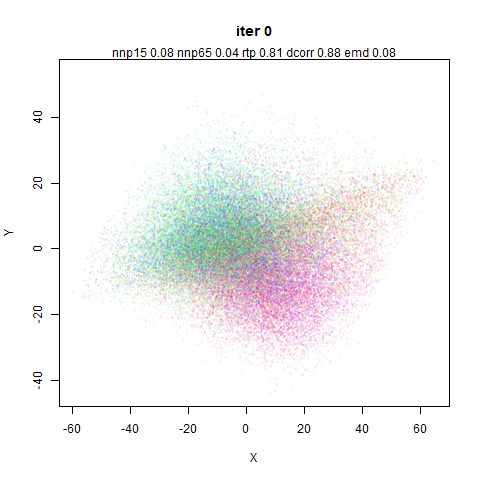
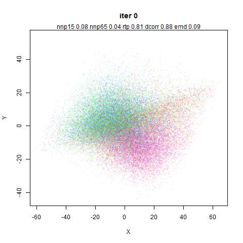
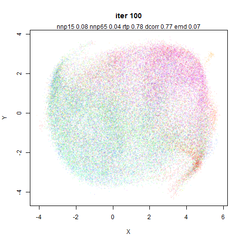
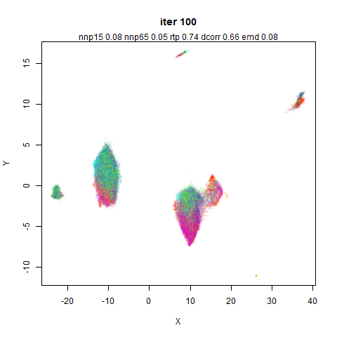
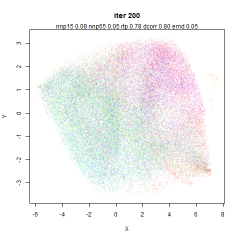
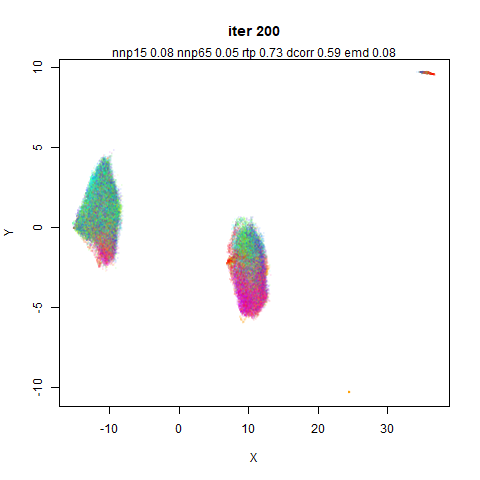
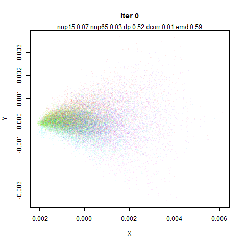
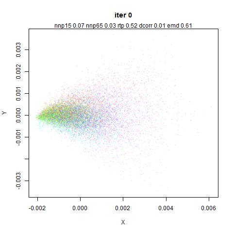
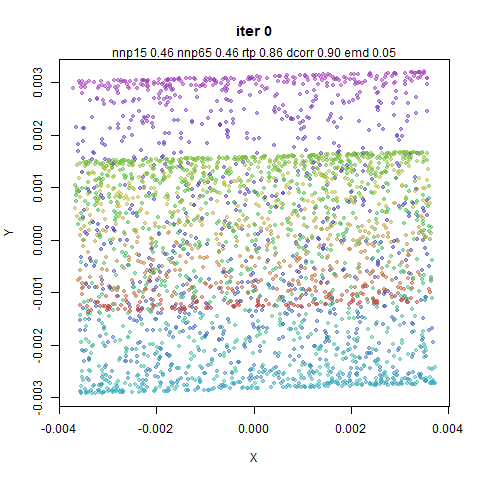
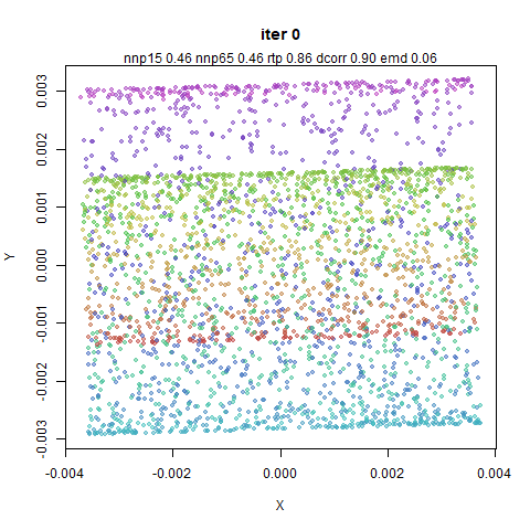
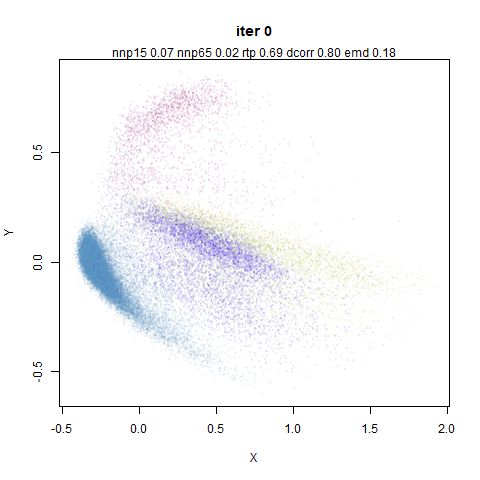
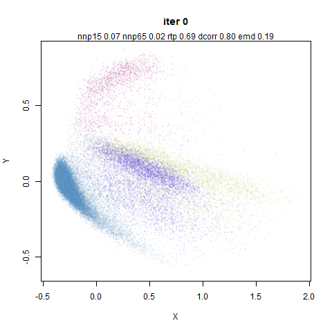
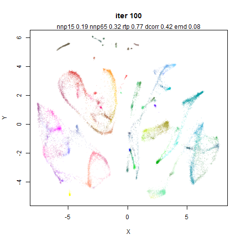
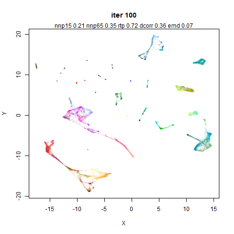
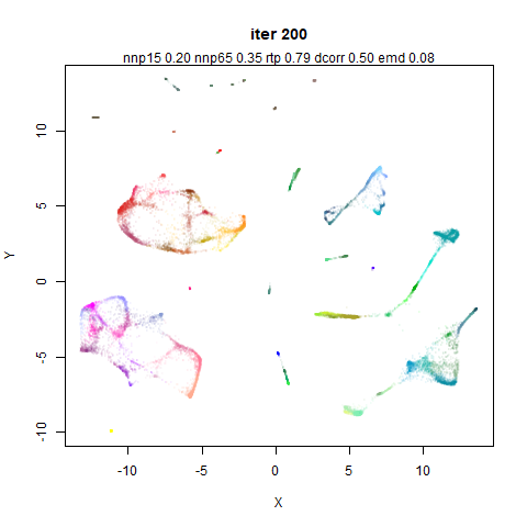
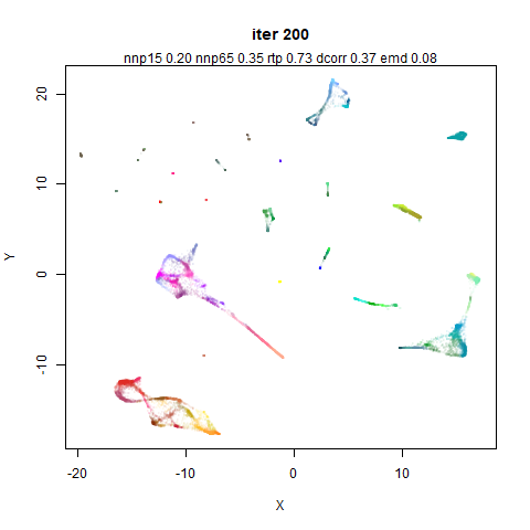
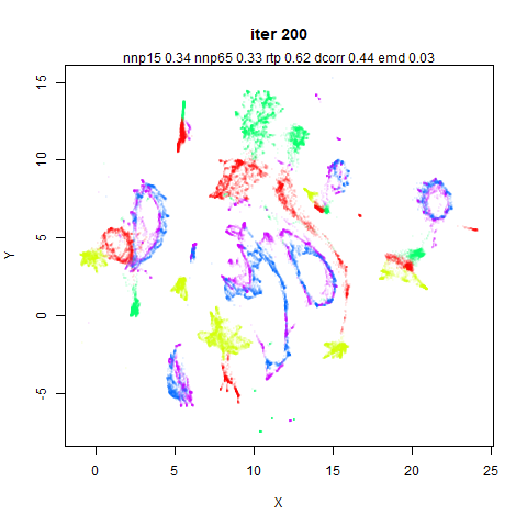
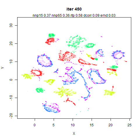
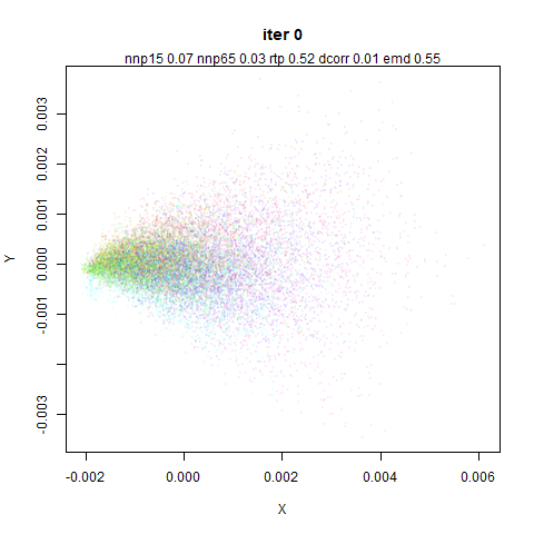
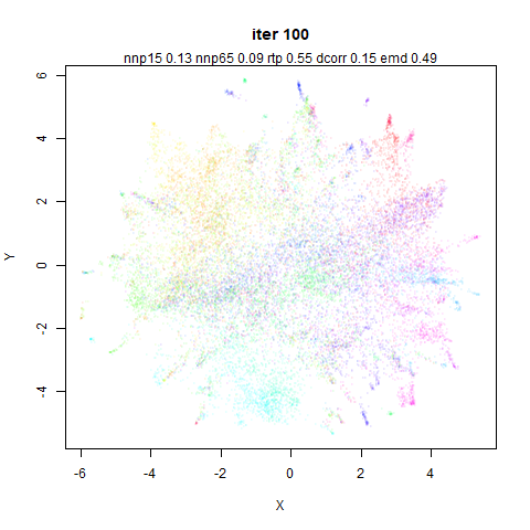
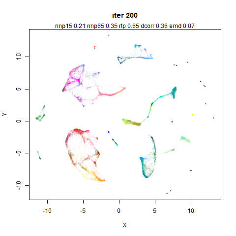
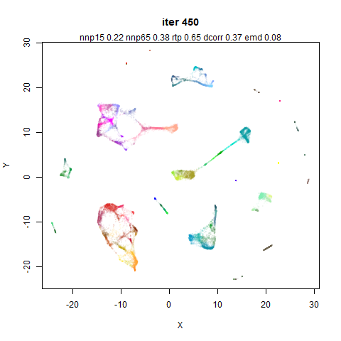
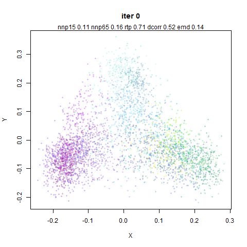
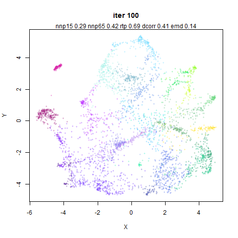
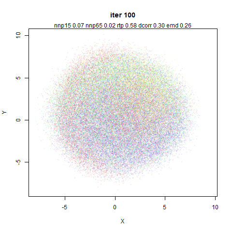
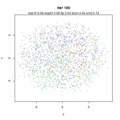
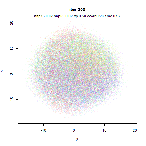
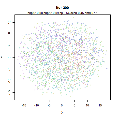
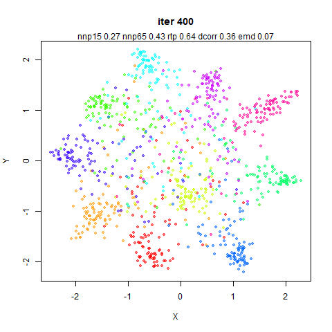
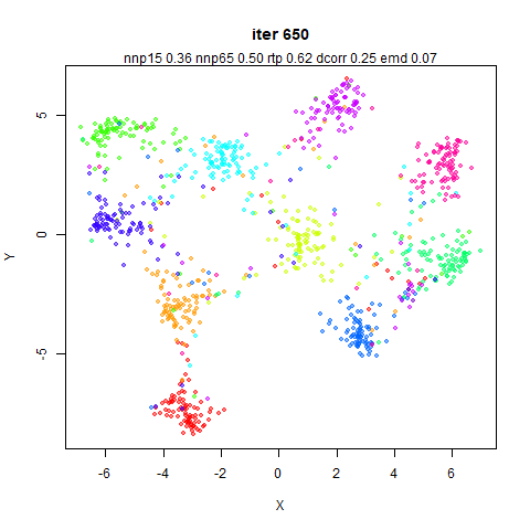
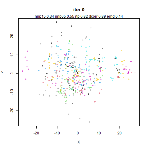
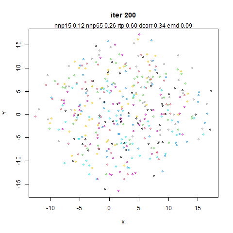
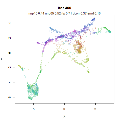
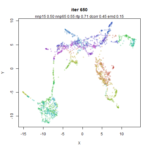
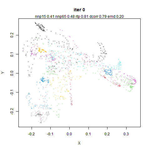
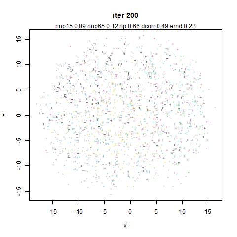
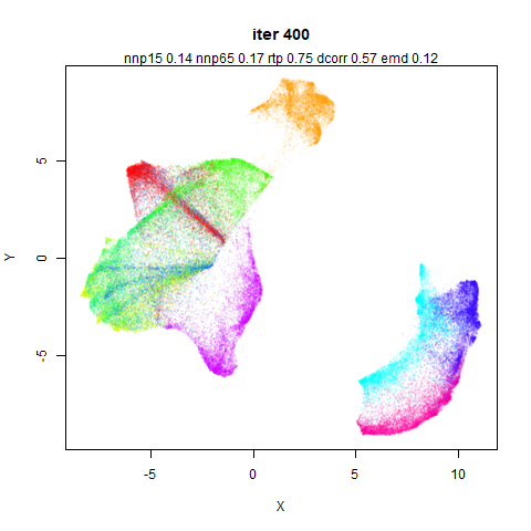
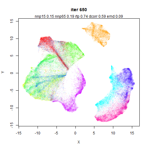
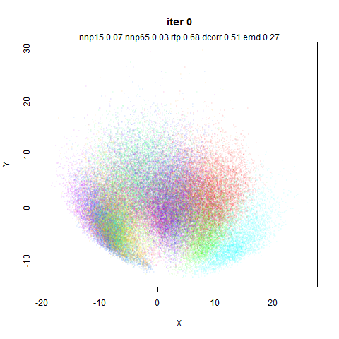
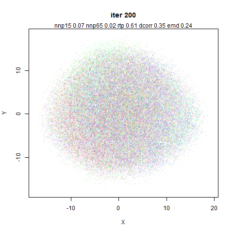
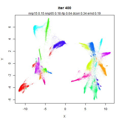
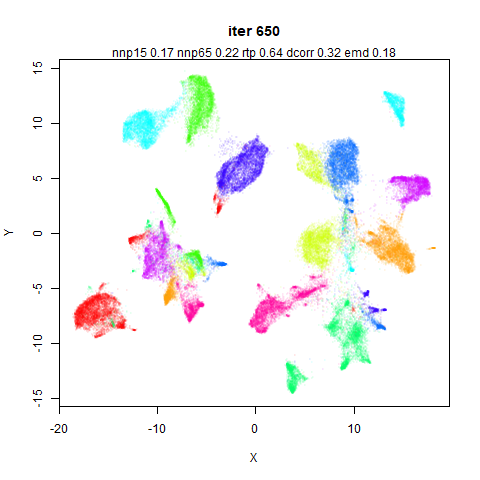
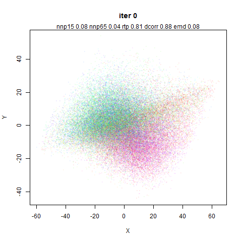
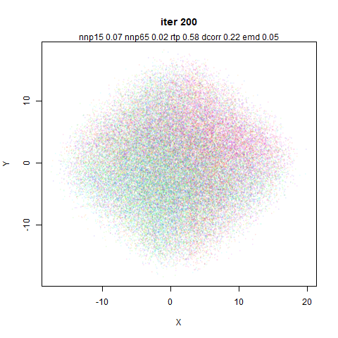
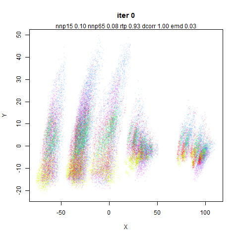
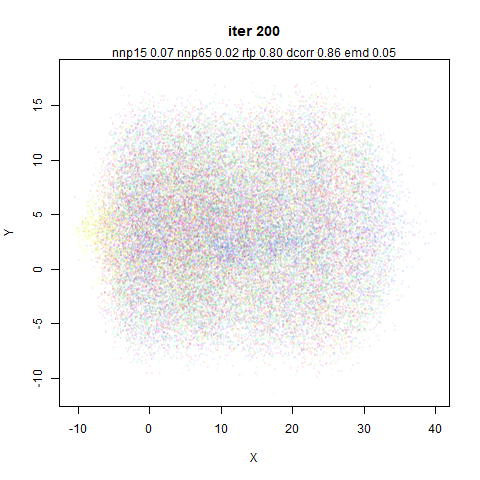
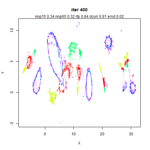
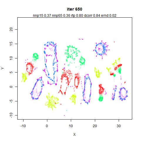
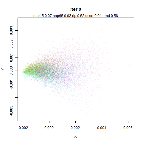
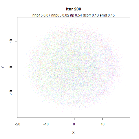
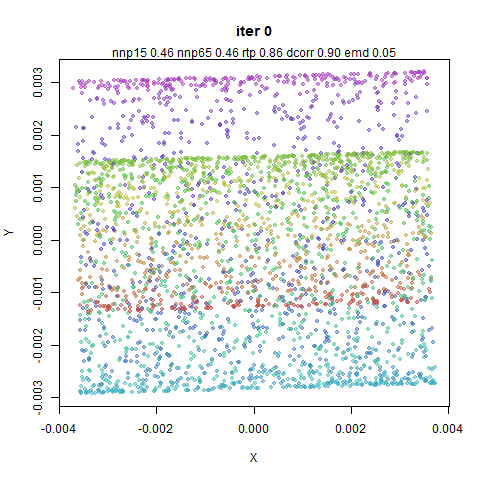
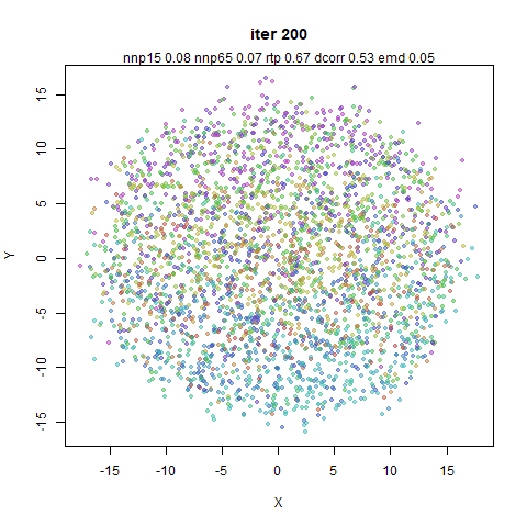
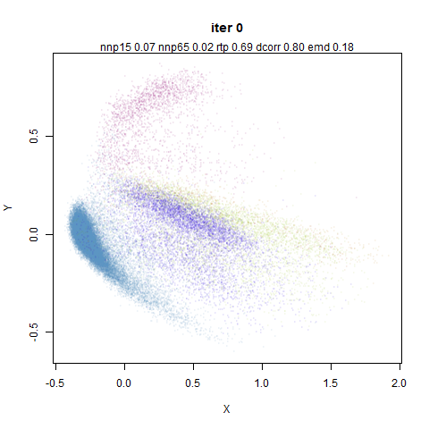
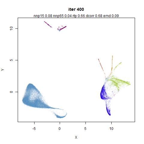
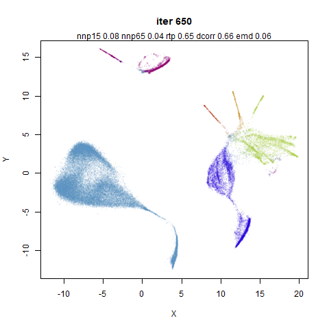
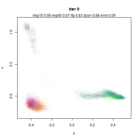
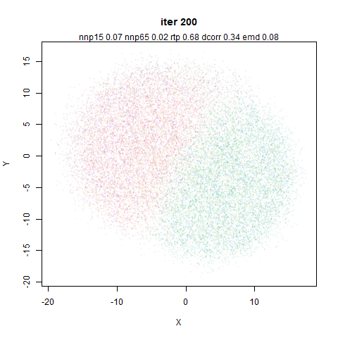
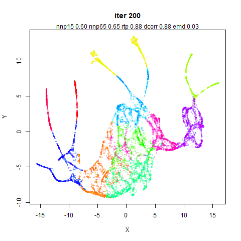
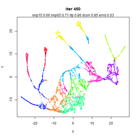
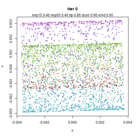
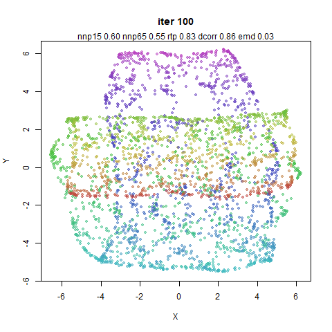
The sub-titles of each plot contain the same assessments of local and
global structure. They are run independently for each set of plots, even
though the 0 iteration is always the same set of coordinates. Any change
in the values represents the natural variance of the stochastic nature
of the evaluation methods. It also depends on the dataset, but variation
in rtp (the triplet preservation) of 0.02
doesn’t seem surprising. Slightly higher changes might be observed for
the emd and dcorr values. I wouldn’t be too
excited about changes smaller than 0.1.
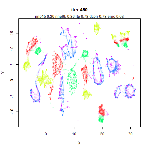
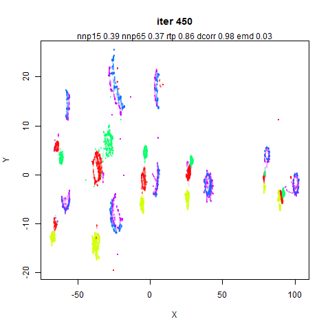
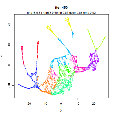
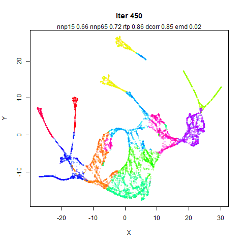
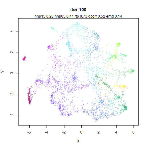
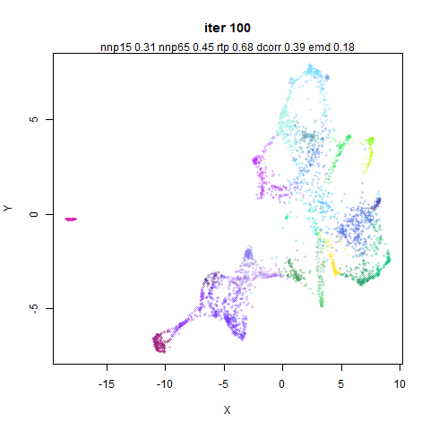
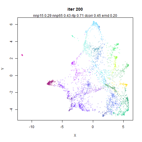
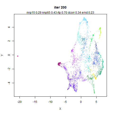
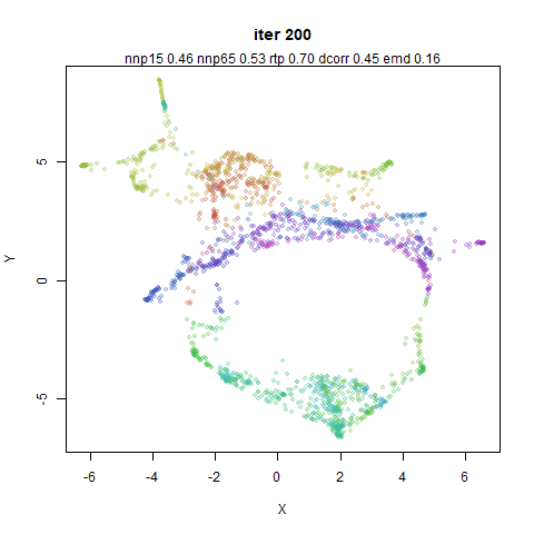
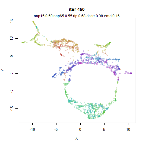
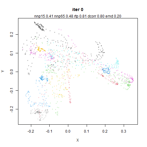
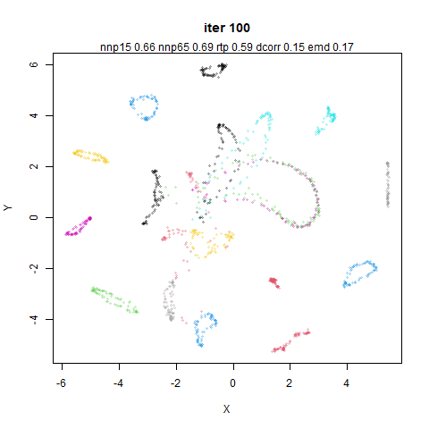
I present most of these images without comment as there is little to
say about most of them. Just soak it in.
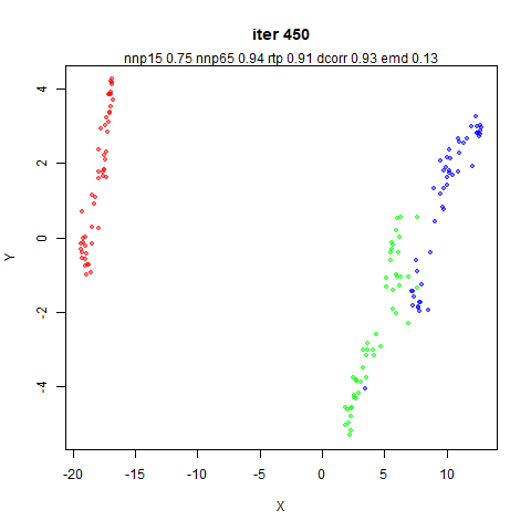
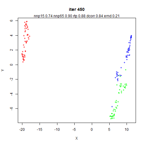
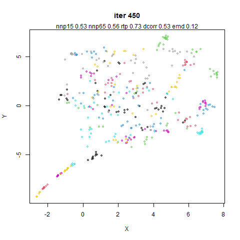
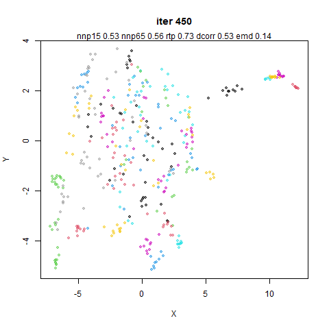
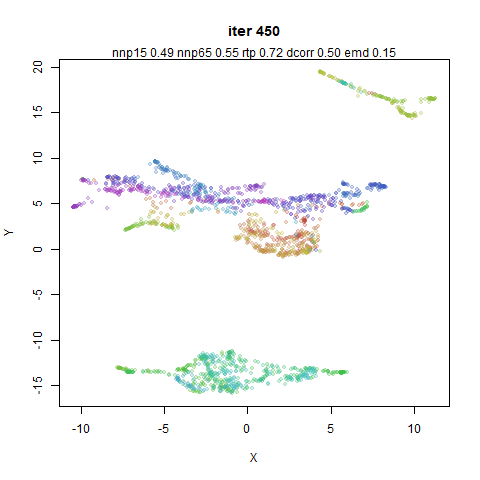
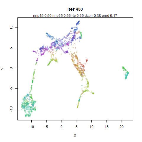
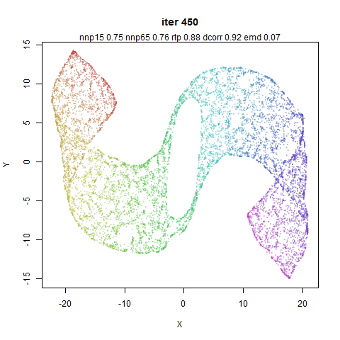
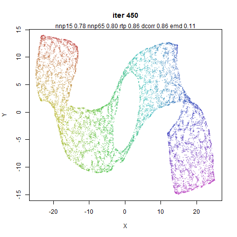
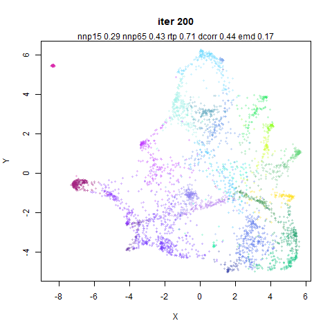
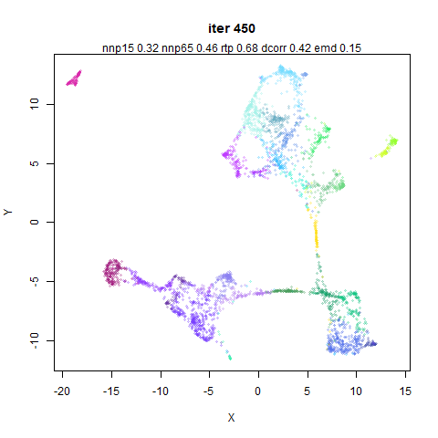
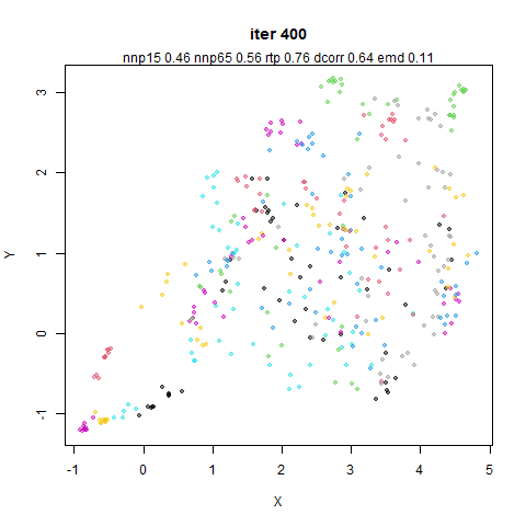
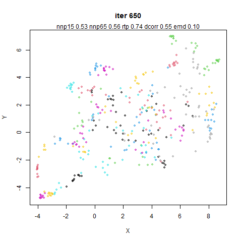
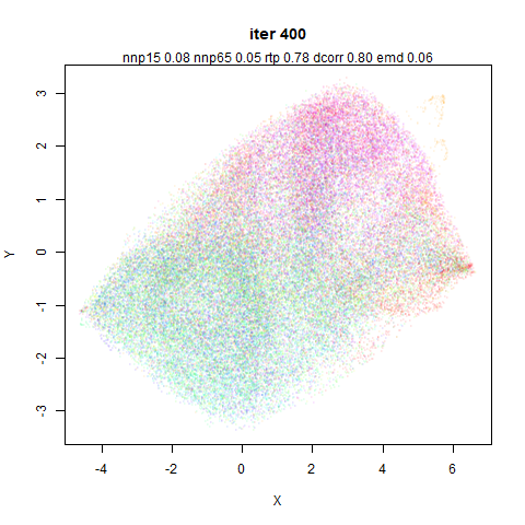
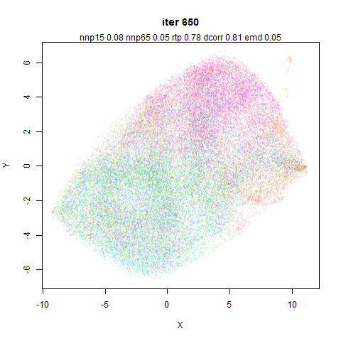
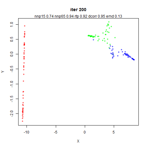
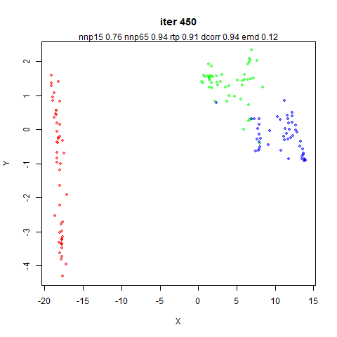
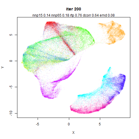
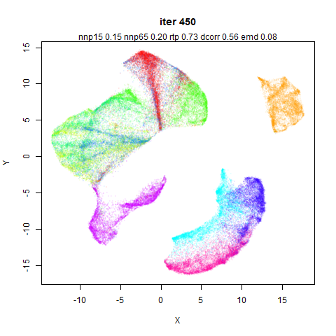
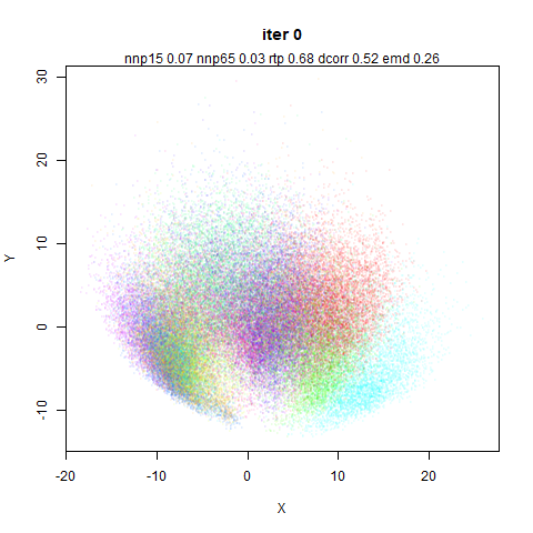
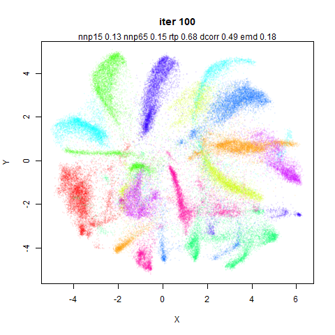
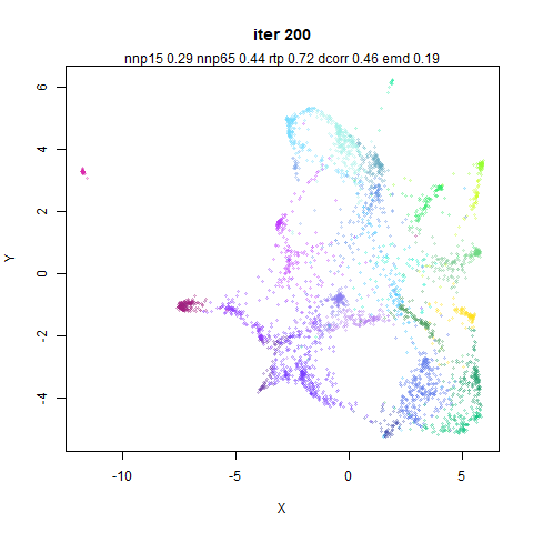
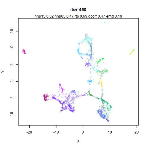
This is one of the few results where there is a noticeable difference
in the visual output and one of the metrics, which favors
retaining the mid-near weighting.
Again, the distance correlation indicates that turning off the
mid-near weights is a mistake.
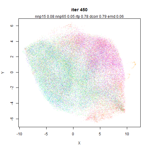
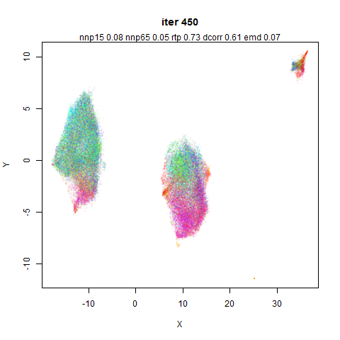
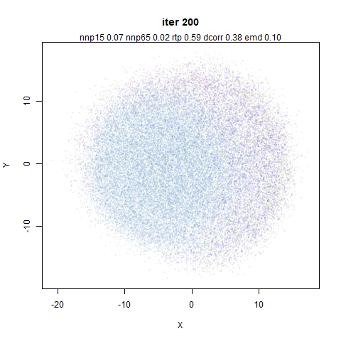
The CIFAR-10 dataset does not embed in an interesting way in any
method I have ever used, but having it split off into three chunks is
definitely not ideal. Again the dcorr metric most strongly
indicates that something has gone wrong.
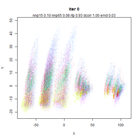
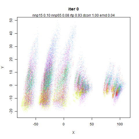
As to why this happens, it must be because of the vary large variance
in the first two principal components, which lead to large inter point
distances which cannot be easily recovered from without the mid-near
points: compare the range of the axes at iteration 0 for this dataset vs
other which are more well-behaved.
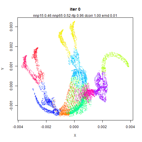
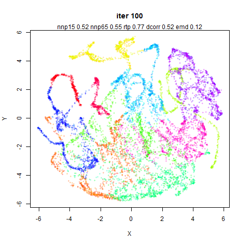
Another dataset where there is a lot of variance in the initial
principal components. It’s clear here that if the initialization is too
diffuse, the different parts of the dataset optimize in isolation from
each other. The global structure metrics indicate that this is a better
embedding than the one that uses mid-near pairs though. Probably global
metrics that stay too close to the PCA results are an indicator of this
sort of thing happening.
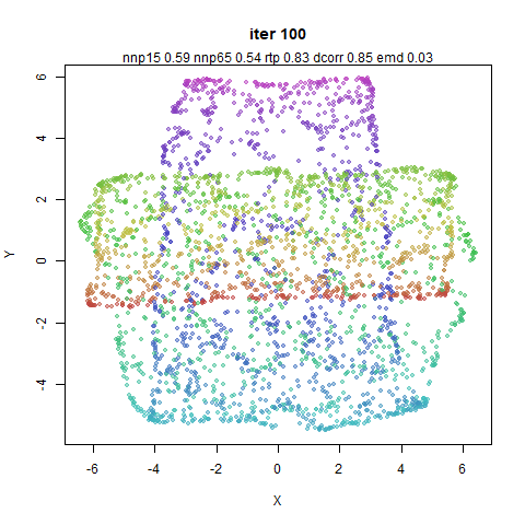
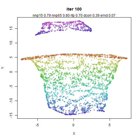
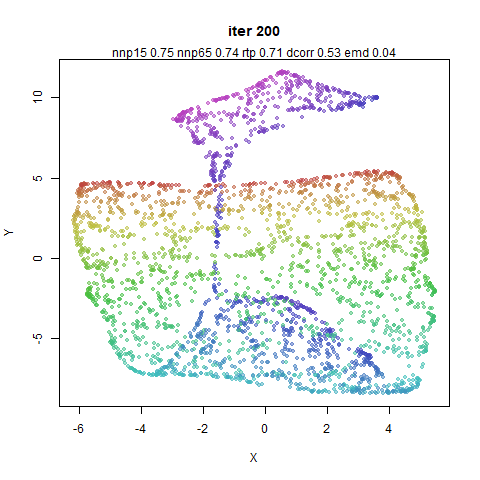
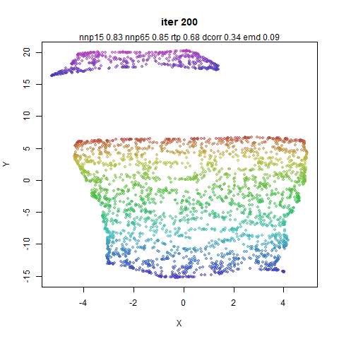
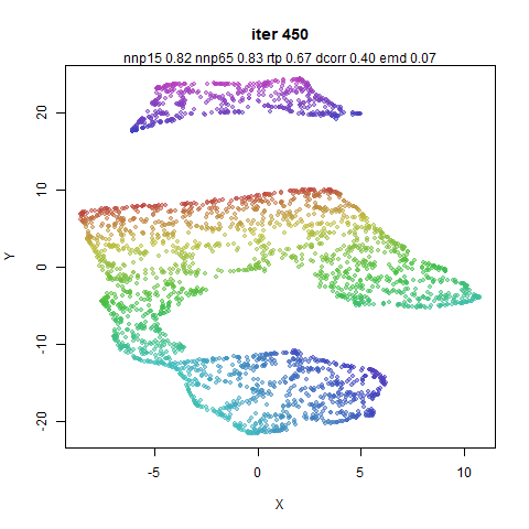
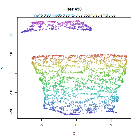
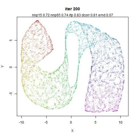
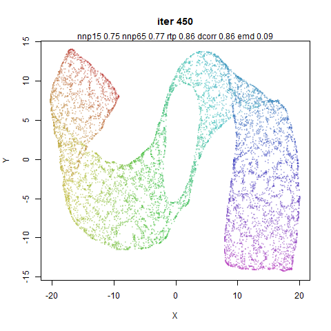
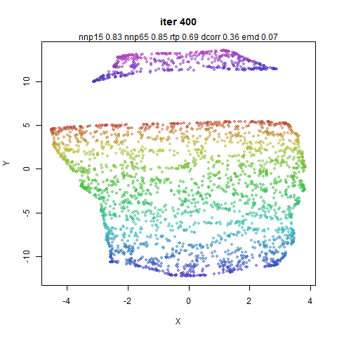
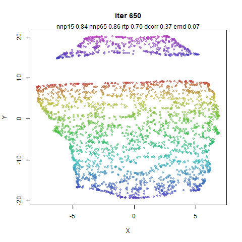
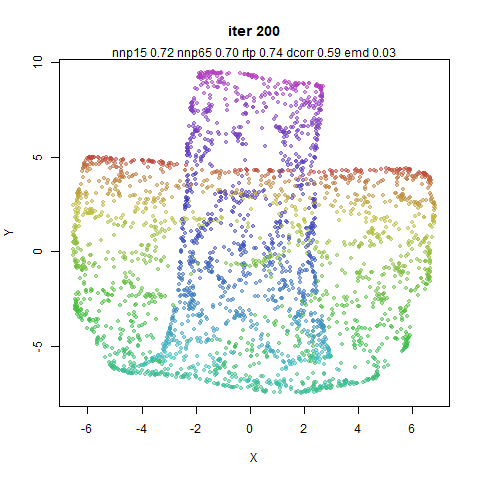
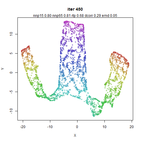
In both cases, the mammoth’s leg has detached from the main body.
dcorr favors keeping the mid-near pairs here.
So for a lot of these datasets, removing the mid-near pairs doesn’t
do much with a PCA-based initialization. This is not surprising. But for
some datasets the metrics (usually dcorr) seems to indicate
that keeping the mid-near pairs around is a good idea, even with a
PCA-based initialization. I think a lot of that could be explained by
the fact that PaCMAP doesn’t try very hard with its initialization. By
fixing the variance of the input to ~1.0, I suspect
datasets like norb and cifar10 would behave
similarly with or without the mid-near pairs.
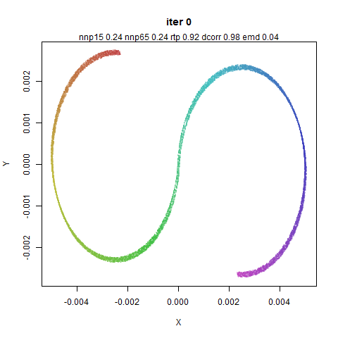
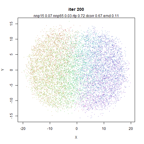
Also of note: the neighborhood preservation metrics are utterly
insensible to the sometimes large global changes in the datasets here.
Invariably, the PCA results always show a fairly low neighborhood
preservation and a high global preservation, and over the course of the
embedding, the neighborhood preservation increases at the cost of the
global distances.
Random Mid-Near Distances
When looking at the distribution of the mid-near distances and random
distances I thought they looked quite close to each other. So can we
just use some random distances instead? Maybe the role of the mid-near
pairs is to keep the overall distribution of distances in a range where
the near pairs can actually be effective?
Below on the left hand column is the same results that you just saw.
Believe me you will not want to be scrolling up and down looking for
these for comparative purposes. On the right hand column is the result
of using random distances instead of the mid-near pairs. Weights were
kept the same as with the “real” mid-near pairs.
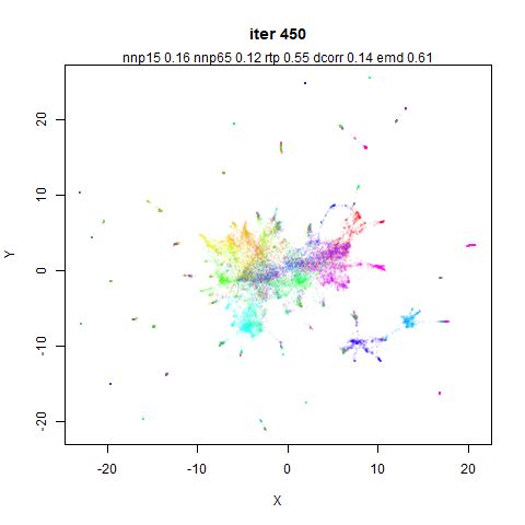
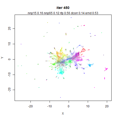
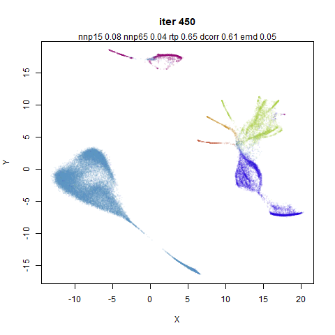
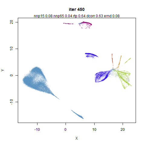
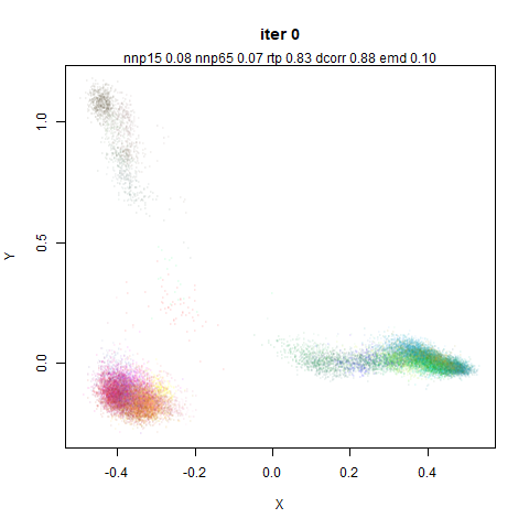
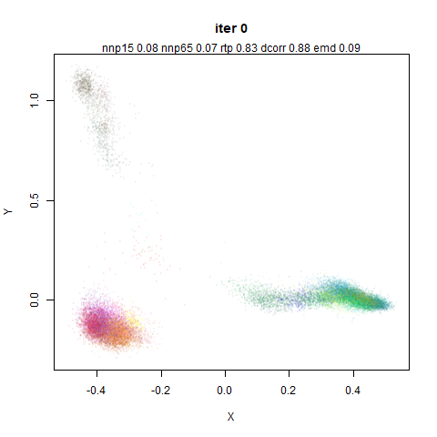
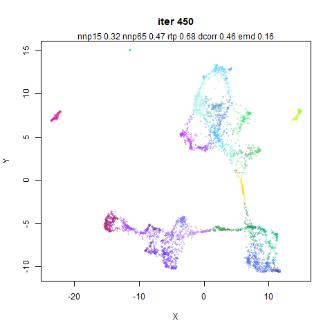
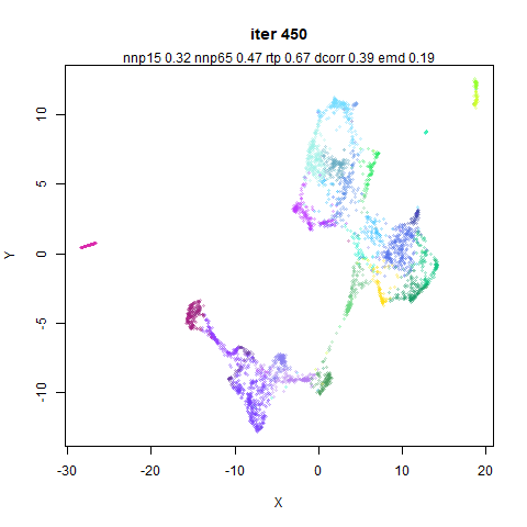
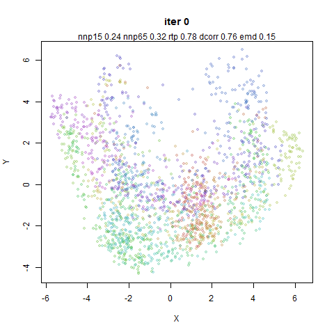
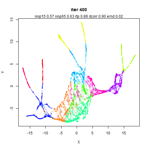
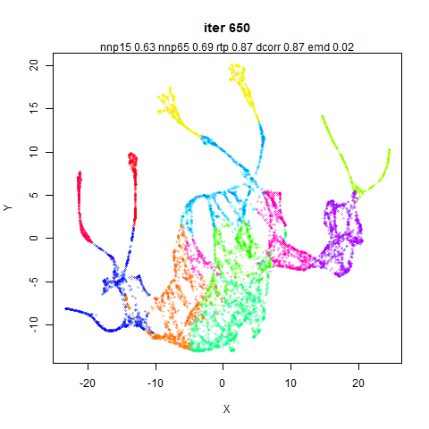
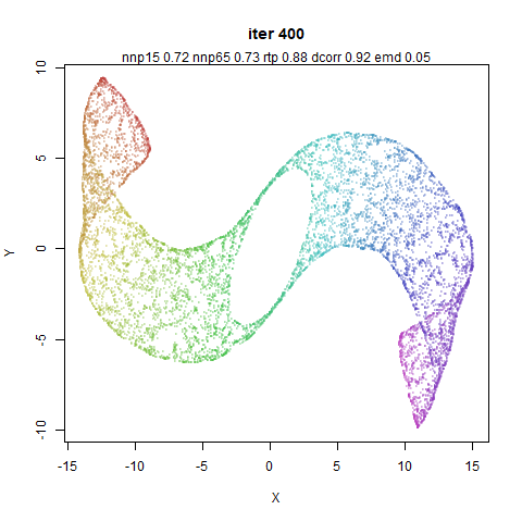
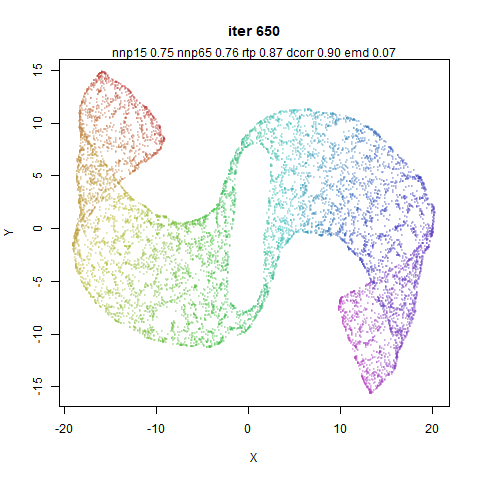
The Frey faces dataset seems to be reliably sensitive, perhaps
because it is more like a manifold than some of the other
(non-synthetic) datasets. Again, mid-near pairs seem to be improve the
global structure.
Ok, so this is actually quite a big effect according to
dcorr and even rtp agrees. The random
distances definitely reduce the global structure here. Visually, I would
have a hard time deciding that the right hand structure was “worse” than
the left hand one in any way.
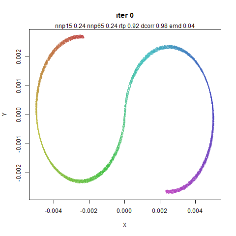
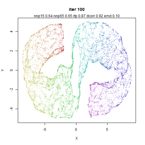
A tusk has been unfortunately snapped off the random distance mammoth
here.
Personally, I think the result from using random distance for the
mid-near pairs is better here. This shows the limitations of the global
measures of structure: you want the manifold to unfold here, which means
the straight-line Euclidean distances should not be
preserved.
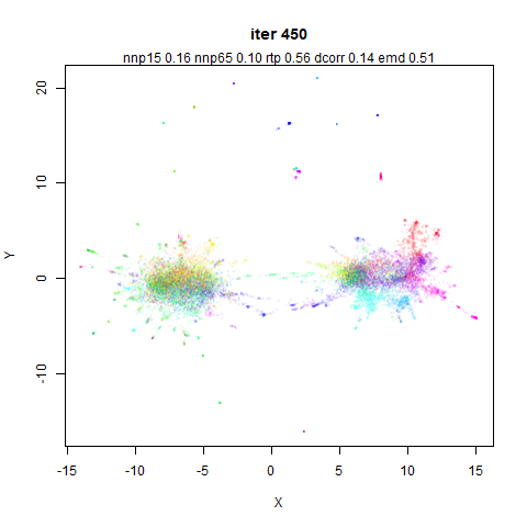
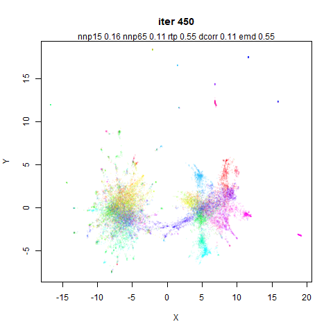
Lots of results here where the dcorr metric was very
clearly showing a difference in these results, and invariably it says
that using uniformly-sampled random distances is a bad idea.
Turning Off Early Near Pairs
I was curious if mid-near pairs could be used exclusively during the
first 200 iterations, without also using the near pairs. Maybe something
like this could be used to initialize other embedding methods like t-SNE
and UMAP if so?
This doesn’t work out too great. Below are two illustrative examples
of what happens using mnist and frey, where I
just set the near pair weights to 0 for the first 200
iterations.
When the near pairs are turned on it looks like they aren’t capable
of pulling neighboring points back together.
Splitting Mid and Near Pairs
The above results give a clue as to why the near pair weight is set
to 2 or 3 during the period of the embedding when the mid-near pairs are
active: they are acting to break up local structure in favor of global
structure so you need a countervailing attractive force to keep the
local structure together.
For the following plots, I turned off the mid-near pair weights for
the first 200 iterations, then for the next 200 iterations turned off
the mid-near weights and set the near-pair weights to 5,
and then had the final 250 iterations as before (with the near-pair
weights set to 1). This effectively splits the first 200
iterations where the mid-near and near pairs are both on, into two
separate 200 iteration sequences, where only one or the other is
present. I found I couldn’t get away with setting the near pair weights
to 3 in this case. As you will see below, without the near
pair attractions acting to compress the embedding initially, the effect
of the mid-near weights is to cause the initial coordinates to be much
more spread out. Hence you need a stronger attractive force to pull them
back in once the mid-near pair forces are turned off.
Also bear in mind that the comparisons between methods here aren’t
for the same number of iterations, the right hand side gets an extra 200
iterations. Although the same number of attractive updates occur in both
cases, the repulsive interactions are always on, so there are 200 extra
iterations worth of repulsive coordinate updates for the images on the
right hand side.
One of the few examples where the dcorr indicates a
difference (in favor of not splitting the different weightings).
In most cases there isn’t much difference between the two methods. So
maybe splitting the mid-pair from the near-pair interactions is a
possible way to get some of the benefits of PaCMAP’s apparent robustness
to different initialization strategies in non-PaCMAP methods. Some
tweaking of the weights seems like it might be needed if you didn’t want
to do some kind of early exaggeration-style over-attraction, but you
might well be doing that with t-SNE anyway.
Using Unscaled Neighbors
I spent a lot of time looking at the effect of local scaling on the
hubness in these datasets. My expectation is that PCA seems to reduce
any hubness such that the effect of local scaling is less likely to have
a noticeable effect.
For this experiment, the right hand column uses the raw 15-nearest
neighbors.
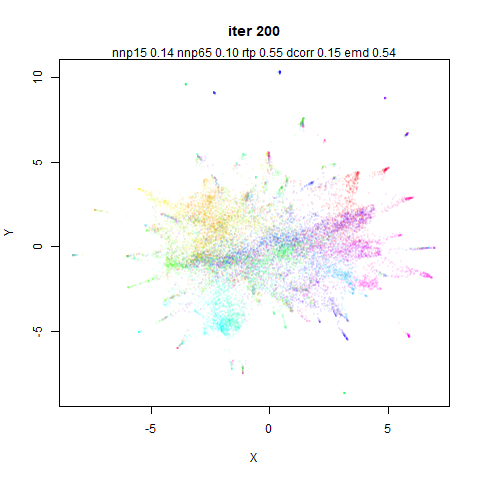
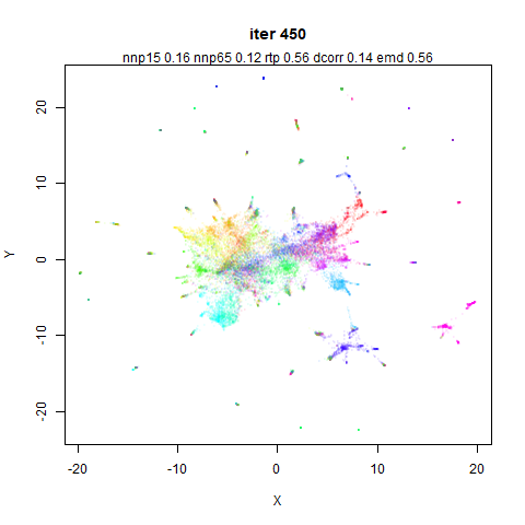
The olivetti faces have a high level of hubness, but I’ve never
really noticed any issues around embedding it with t-SNE, UMAP and now
PaCMAP. So despite the local scaling being very effective at reducing
hubness, I am not very surprised that visually I don’t see a huge
difference.
CIFAR-10 is one of the datasets where local scaling substantially
reduces hubs but I was not holding out much hope for a big change. And
basically nothing happens.
In terms of the effect of local scaling, 20NG is affected a lot like
CIFAR-10. And it shows the same disappointing lack of much going on.
There is at least a slightly different tearing of the manifold than
we see for the other changes carried out in this document. Again the
state of the embedding is not as bad the disparity in dcorr
suggests (if anything the opposite).
This is the final dataset that I thought I might see some changes
with local scaling. The dcorr does go up but not by much.
Given the emd shows an increase (that’s a bad thing) I
would be hard pressed to say my expectations were met.
I wasn’t expecting much to happen and it didn’t. At least with
n_neighbors=15, and all the other settings as defaults, I
am not sure that local scaling is actually worth the effort here. Maybe
it’s helpful with a different initialization?
PCA/Scaled Neighbors
Ok, so local scaling doesn’t seem to do much to the datasets above,
but we’ve seen that carrying out PCA can have a big effect on the input
distances. What if local scaling proves its worth when PCA isn’t carried
out (with apply_pca=False)?
I focus here on the two datasets where local scaling has a big effect
on the neighborhoods: macosko2015 and ng20.
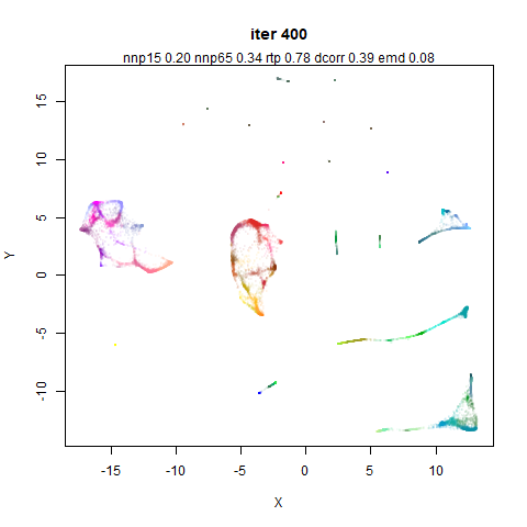
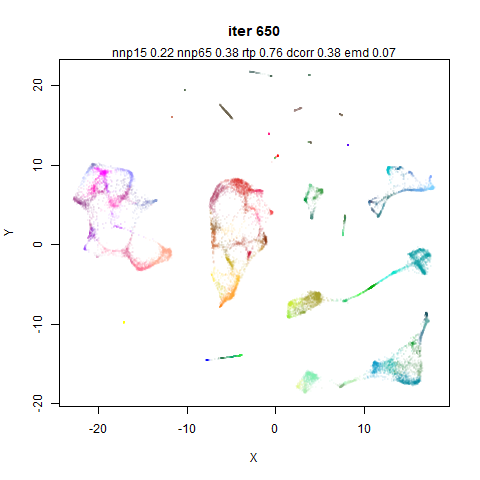
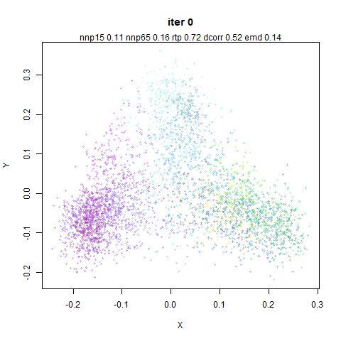
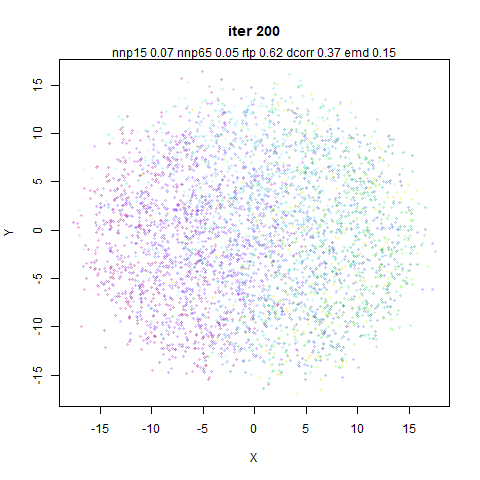
cifar10 might also have an effect but we have already
established that it just sits there like a big useless lump so let’s not
waste time on that.
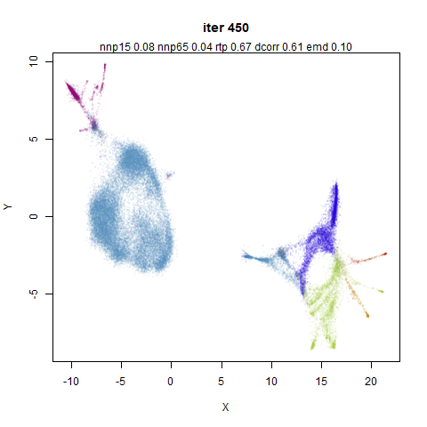
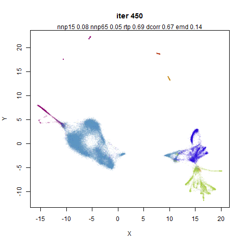
Below are four images for each dataset, the final coordinates after
450 iterations. The top row uses the approximate 15 nearest neighbors
without local scaling. Top left doesn’t use PCA (so is like the sort of
nearest neighbors UMAP would use). Top right applies PCA (so is the same
figure as used in the final row of the previous section’s tables). The
bottom row is for the scaled neighbor results: bottom left does not
apply PCA. Bottom right does apply PCA, so is the standard PaCMAP
results we have been comparing all along.
Also: I also turned off the scaling for the non-PCA case, where the
data is scaled between 0 and 1 before centering. The data is still
centered, so it’s more comparable to the PCA case, where the data is
also centered, but not scaled before applying PCA.
The non-PCA results definitely look different to the PCA results,
thus vindicating my strong recommendation not to blindly apply PCA to
your data for pre-processing. And the local scaling might be having more
of an effect than in the PCA case. It would be fair to say that it
doesn’t seem to do much, though. The metrics don’t seem to be hugely
affected either.