HSSNE

This article retains its original experiments and examples. For current package usage, see the usage guide.

HSSNE is an embedding method that generalizes SSNE and t-SNE, by introducing an alpha parameter into the output weight function. When it’s set to 1, it gives the t-SNE results. As it approaches zero, it gives the SSNE results. Values between 0 and 1 therefore give a result where the amount of “stretching” is intermediate between SSNE and t-SNE. Values of alpha greater than one correspond a stretching of the output distances that is greater than that provided by t-SNE.

On the face of it, there’s no reason to believe that all datasets are best served by a value of alpha = 1, which is what using t-SNE does implicitly. Some datasets need less stretching (this certainly seems to be the case with iris), and maybe some need more.

The heavy-tailed output kernel is defined as:

w_{ij} = \frac{1}{\left(\alpha d_{ij}^2 + 1\right)^{\frac{1}{\alpha}}}

with d_{ij}^2 being the squared output distance. It’s easy to see that the t-distributed kernel is recovered when \alpha = 1. You may have to take my word for it that this becomes the Gaussian kernel as \alpha \rightarrow 0 (or plot it).

December 29 2019: HSSNE is also implemented in FIt-SNE, although in the associated paper the degree of freedom parameter, while also referred to as \alpha, is defined as 1 / \alpha compared to the original HSSNE. So when comparing their recommended values with those tried here, take the reciprocal of their reported values.

Gradient

The HSSNE gradient is:

\frac{\partial C}{\partial \mathbf{y}_i} = 4 \sum_j \left( p_{ij} - q_{ij} \right) w_{ij}^\alpha \left( \mathbf{y}_i - \mathbf{y}_j \right)

Datasets

See the Datasets page.

Evaluation

Apart from visualizing the results, the mean neighbor preservation of the 40 closest neighbors is used to provide a rough quantification of the quality of the result, labelled as mnp@40 in the plots.

Settings

Here’s an example of generating the results using the iris dataset and choosing a non-default value for alpha. The default value for alpha is 0.5, which is arbitrary, but sits between SSNE and t-SNE settings.

iris_hssne1_5 <- smallvis(
  iris,
  scale = FALSE,
  perplexity = 40,
  Y_init = "spca",
  method = list("hssne", alpha = 1.5),
  ret_extra = c("dx", "dy"),
  eta = 10
)

Results

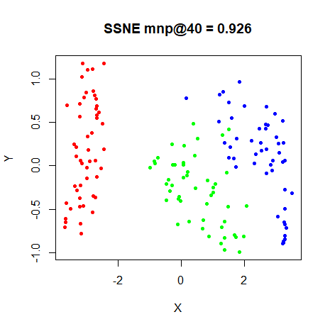
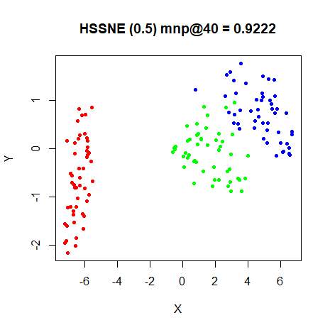
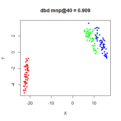
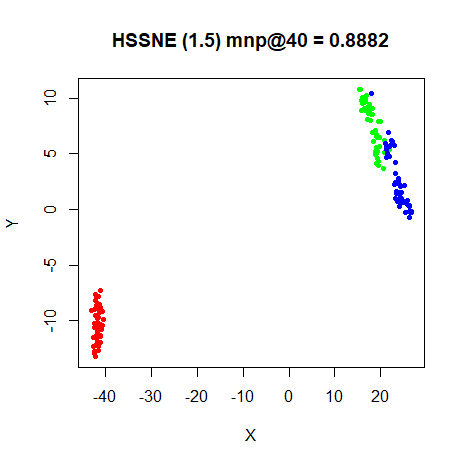
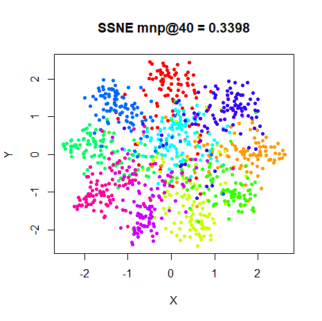
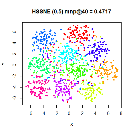
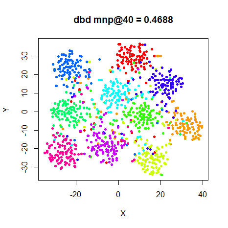
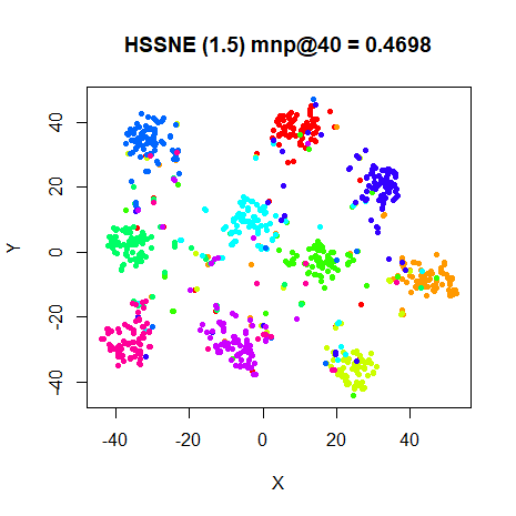
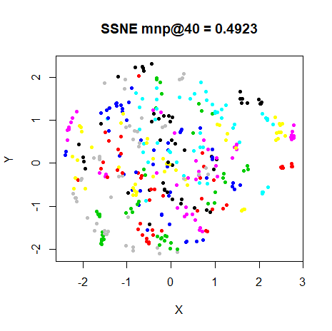
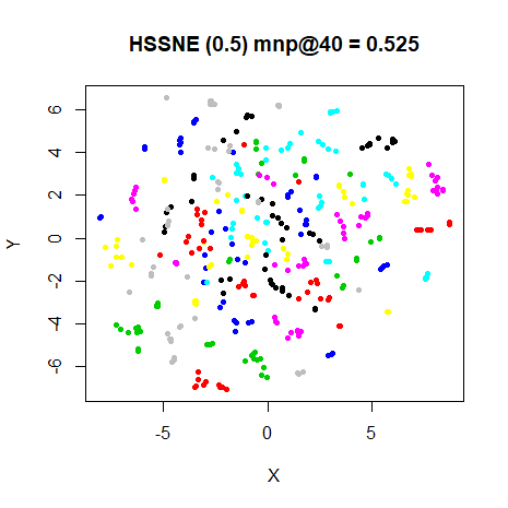
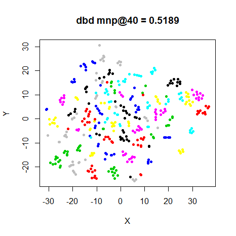
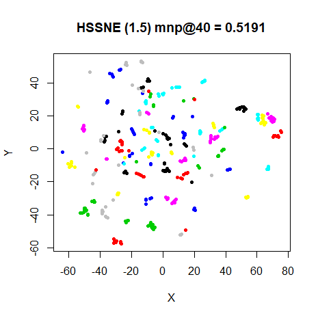
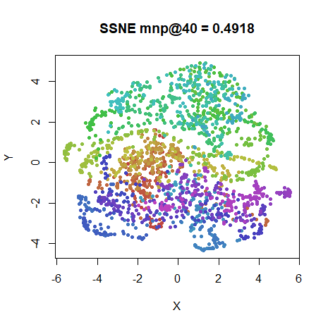
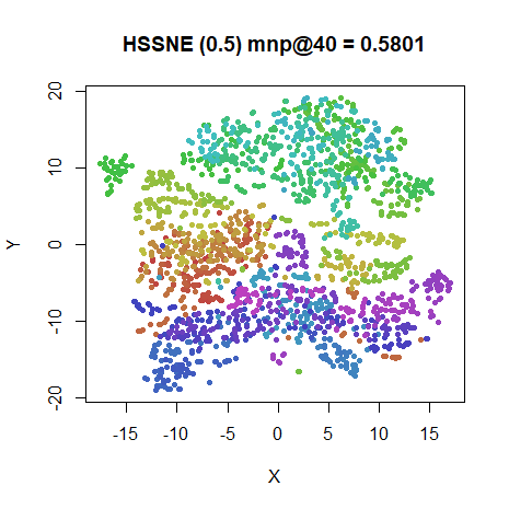
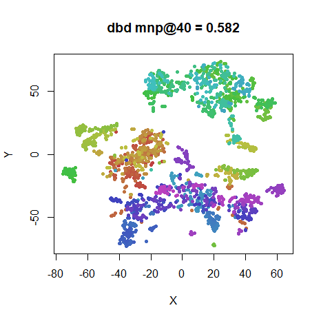
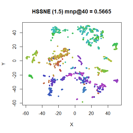
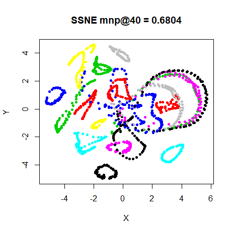
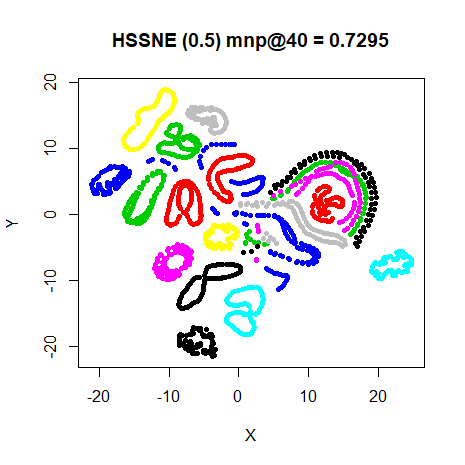
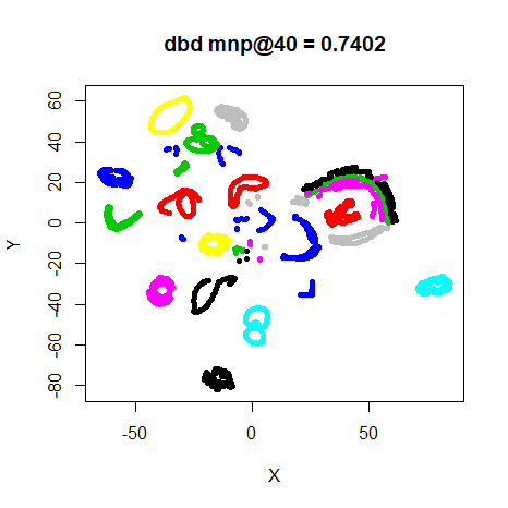
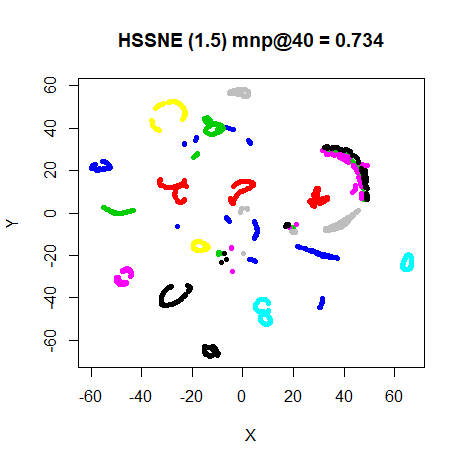
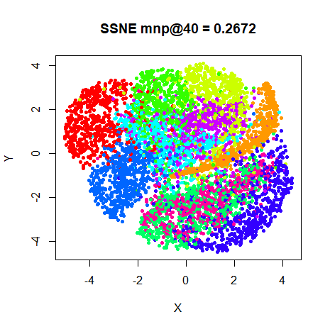
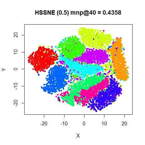
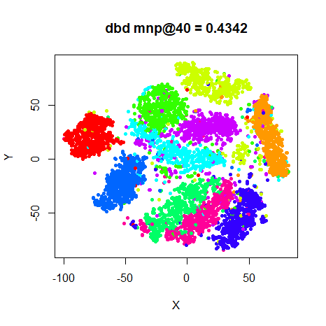
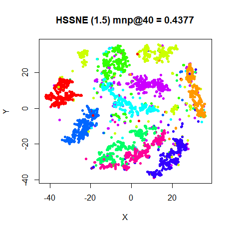
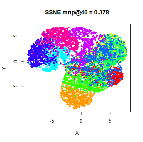
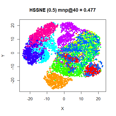
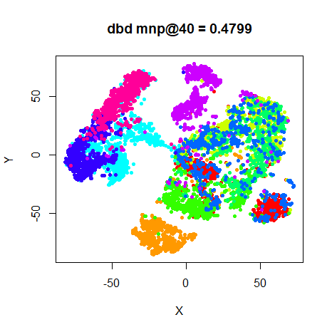
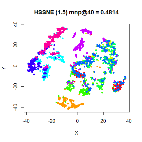
The effective value of alpha increases from left to right and top to bottom in the images below. Top left is the SSNE results, which corresponds to alpha = 0. Top right is alpha = 0.5, a setting half way between SSNE and t-SNE. Bottom left is t-SNE results, which corresponds to alpha = 1. Bottom right is alpha = 1.5, so allowing the distances to stretch even more than t-SNE does.

iris

s1k

oli

frey

coil20

mnist

fashion

Conclusions

The effect of increasing \alpha is quite obvious: compressing the natural clusters that are present in the results. In some of the cases, an \alpha value different from 0 (equivalent to SSNE) or 1 (t-SNE) does give a superior neighborhood retrieval value. But the difference isn’t huge and visually I’m not sure you’d be misled by just using t-SNE in all cases. It may well be that better results could be found by a more fine-grained search of an \alpha value for each data set, but it’s hard to argue for adding another parameter that needs fiddling with, especially given that the presence of the \alpha power in the gradient slows down the gradient calculation compared to t-SNE.

Of course, if there was a way to optimize \alpha, that might be more interesting. There’s certainly a way to do this: a similar strategy was used by van der Maaten for parametric t-SNE. Update February 8 2018: smallvis now offers offers a simple version, which I have dubbed dynamic HSSNE (DHSSNE). You can read more about its performance here.

Extending this idea would be to use a per-point \alpha value, rather than one global value, which would allow different cluster densities to expand at different rates. This definitely would require optimization. Such a technique was described by Kitazono and co-workers and named inhomogeneous t-SNE.

Update December 29 2019: Results by Kobak and co-workers using HSSNE implemented in FIt-SNE and therefore able to study larger datasets (e.g. the entire MNIST dataset) recommend values of \alpha as large as 2 for larger datasets, but note that the optimization effort can be substantially increased. Kahloot and Ekler recommend \alpha = 2.5 for the small NORB and CIFAR 10 and 100 datasets.

January 12, 2018