Dynamic HSSNE

February 8, 2018

This article retains its original experiments and examples. For current package usage, see the usage guide.

This article is a sequel to the testing of the Heavy-Tailed SSNE method. In brief, HSSNE generalizes SSNE and t-SNE by means of a heavy-tail parameter, \alpha. At \alpha = 0, it behaves like SSNE, and at \alpha = 1, it behaves like t-SNE.

In the conclusion of that article, I mention that the parametric t-SNE method suggests that we could optimize \alpha along with the coordinates to get improved embeddings. Parametric t-SNE calculates the gradient of the cost with respect to \alpha (the definition of \alpha in that paper is different from that of HSSNE but they do basically the same thing) and then presumably optimizes \alpha at each step of optimization.

For more on the gradients involved in optimizing the heavy-tail parameter, see here. Doing this in smallvis complicates the code in a way I don’t want to commit to, so I suggest a simpler method:

1. At every epoch, calculate the error for the current coordinates at the current value of \alpha. This already happens anyway if verbose = TRUE.

2. Repeat the error calculation at a value of \alpha \pm 0.1, e.g. if \alpha = 0.5 also look at \alpha = 0.4 and \alpha = 0.6. Candidates must satisfy \alpha \ge 10^{-8}, the implementation’s positive lower bound.

3. If either of these values of \alpha give a lower error, switch to the value of \alpha that most reduced the error and continue the optimization.

In this way, \alpha is allowed to drift from its initial value, and hopefully arrive at a stable value that reflects the data’s natural degree of stretching. This won’t be as accurate as doing a proper optimization and using the gradient, but the results based on manually choosing a fixed value of \alpha didn’t suggest we are going to see a massive change in visualization anyway, so a resolution of 0.1 seems fine to me. My main interest is to see if low-dimensional datasets such as iris and the Swiss Roll end up at lower values of \alpha compared to things like mnist and fashion.

For the starting value of \alpha, I use the default value of 0.5 in these experiments. This seems like a reasonable half-way point between ASNE and t-SNE. Initial experiments using alpha = 0 found that the value of \alpha never changes under these circumstances. Probably, the points end up too crushed together too early and alpha ends up trapped in a local minimum. Using alpha = 1 tended to also end up at the same values as starting at alpha = 0.5 and given that t-SNE works better than ASNE, that might be a better starting point for most datasets, but as I say, it probably doesn’t matter that much, as long as the value of \alpha has the chance the change a bit.

Finally, we need to decide on how often to allow \alpha to change. The more often the change is allowed, the quicker \alpha will (hopefully) reach a good value that will allow the optimization to proceed with the spacing out the clusters in the data correctly, but doing so requires two extra cost evaluations, so we don’t want to overdo it. I chose to set epoch = 50 entirely empirically.

Datasets

See the Datasets page.

The Swiss Roll will also make an appearance here, because it’s easy to see the difference between an ASNE embedding (which looks decent) and a t-SNE embedding (which tears the manifold into small pieces). The it-SNE paper also uses this and successfully unrolls it, so DHSSNE has a fighting chance also. See the Swiss Roll and SNE page for more on that dataset. For these experiments I use a 3,000 point version similar to that used in the inhomogeneous t-SNE paper:

sr3k <- snedata::swiss_roll(n = 3000, max_z = 30)

Evaluation

Apart from visualizing the results, the mean neighbor preservation of the 40 closest neighbors is used to provide a rough quantification of the quality of the result, labelled as mnp@40 in the plots.

Settings

We will compare the DHSSNE with t-SNE results. To account for the fact that we will probably be spending a portion of the DHSSNE optimization at a non-optimal value of \alpha, I used double the number of iterations (compared to default settings) to max_iter = 2000. As mentioned above, I set epoch = 50, so that the value of \alpha can change every 50 iterations.

Finally, I used the Laplacian Eigenmap initialization instead of the scaled PCA results I usually use, just to mix things up a bit, but it does help unfold the Swiss Roll.

iris_dhssne <- smallvis(
  iris,
  method = "dhssne",
  Y_init = "lap",
  scale = FALSE,
  epoch = 50,
  perplexity = 40,
  eta = 100,
  max_iter = 2000,
  ret_extra = c("alpha")
)
iris_tsne <- smallvis(
  iris,
  method = "tsne",
  Y_init = "lap",
  scale = FALSE,
  epoch = 50,
  perplexity = 40,
  eta = 100,
  max_iter = 2000
)

Results

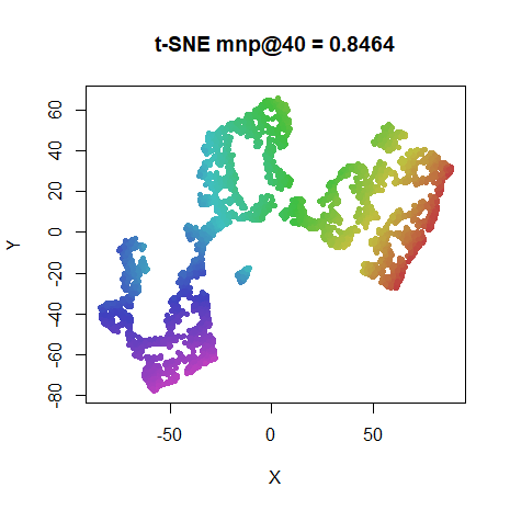
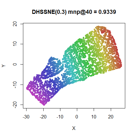
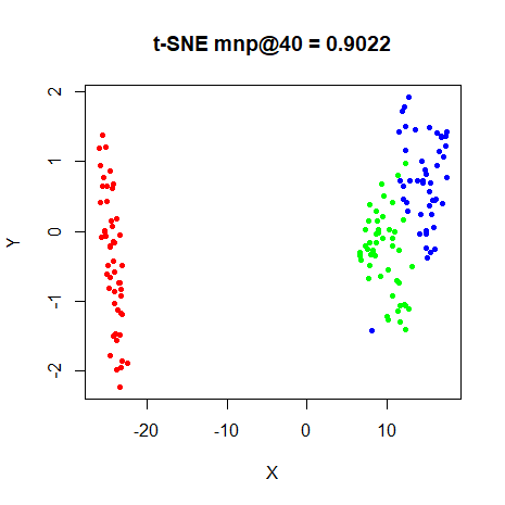
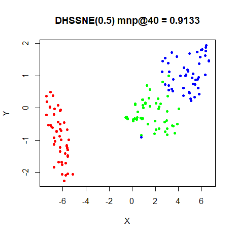
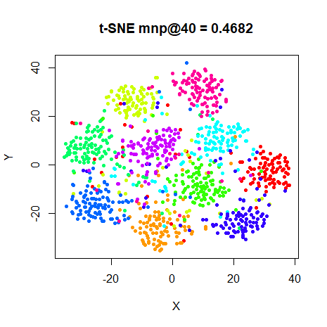
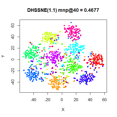
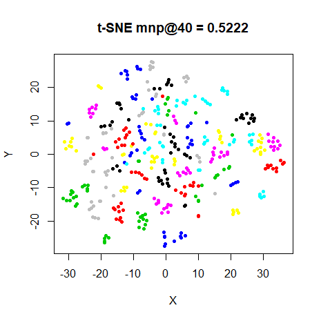
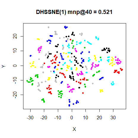
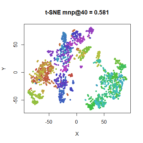
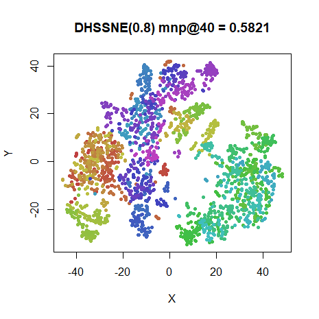
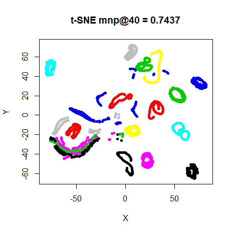
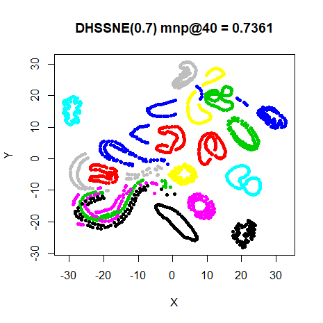
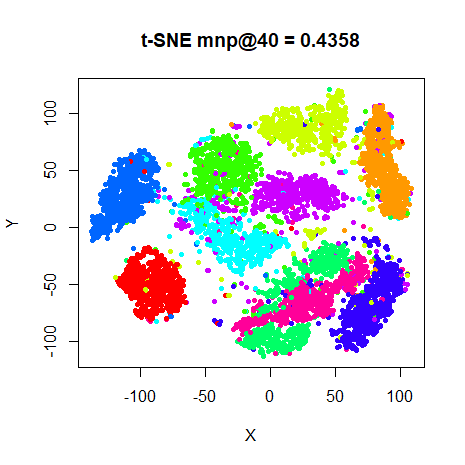
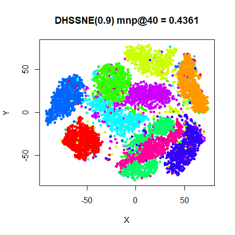
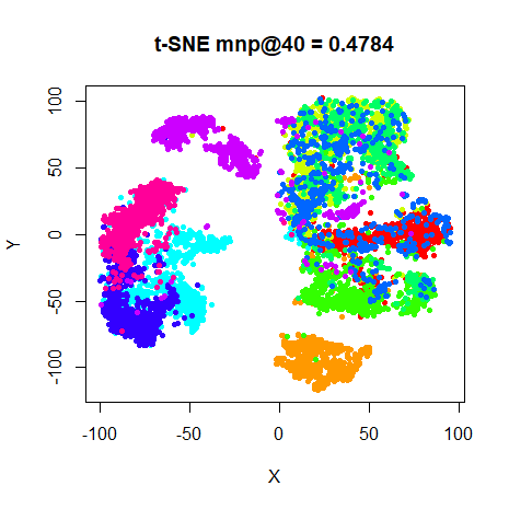
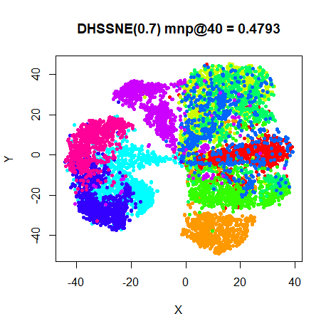
For each dataset, the left-hand image below is the t-SNE result. The right-hand image is the DHSSNE image. The number in parentheses in the title is the final value of \alpha used for that dataset.

swiss

iris

s1k

oli

frey

coil20

mnist

fashion

Conclusions

The Swiss Roll is the big winner with DHSSNE, which looks much better than with t-SNE. Unfortunately, none of the other datasets benefit. Only s1k ends up at an \alpha \gt 1, although all the datasets end up with \alpha \ge 0.5. However, the neighborhood preservations are basically unchanged, with coil20 and iris seeing the biggest change. Visually, coil20 is probably the most affected, and I’d say the t-SNE result is to be preferred there. For the other datasets the overall structure of the embedding is not affected, but there is less spacing of any clusters, as expected from using a lower \alpha. This might better reflect the underlying probability distribution that is being modelled, but as t-SNE is mostly a visualization tool, there is usually a bias to seeing more spacing between clusters, so t-SNE is still to be preferred here.

Finally, DHSSNE is slower than HSSNE which in turn is slower than t-SNE. I suspect the slower behavior of DHSSNE is due to some copy-on-write of the internal data structures used in smallvis when the value of \alpha is updated, so that can be improved, but the simpler gradient of t-SNE compared to HSSNE will be fundamentally faster even without those issues.