opt-SNE settings

February 25, 2019

This article retains its original experiments and examples. For current package usage, see the usage guide.

For large datasets, particularly those using biological data, Belkina and co-workers came up with a series of guidelines about how to better separate clusters, which is part of their opt-SNE code. There are three main suggestions:

• The learning rate (eta in smallvis) should be data dependent, and can be much larger than the usual defaults of 100-250 for large datasets. They recommend a value of N / \alpha where N is the number of objects in the dataset, and \alpha is the early exaggeration factor (usually 12 for larger datasets).

• Early exaggeration may need to be run for substantially longer than usual. Rather than stop early exaggeration after a fixed number of iterations, they suggest monitoring the relative rate of change of the KL divergence, (\mathrm{KL}_{i-1} - \mathrm{KL}_{i}) / \mathrm{KL}_{i-1}, and terminate early exaggeration after it reaches a maximum. Normal optimization then proceeds for the rest of the iterations available. In the paper, an example is given where optimal results were obtained after 750 iterations of early exaggeration, followed by another 750 iterations of standard optimization.

• Because early exaggeration can last a longer than usual, it might be tempting to keep the ratio of early exaggeration iterations to standard optimization iterations, e.g. 75%-90% of the total number of iterations should be non-exaggerated. But because the early exaggeration is extended, this would in turn lead to a very long run time for the standard optimization. Instead, the authors suggest monitoring the relative tolerance of the KL divergence, and terminate the run when \mathrm{KL}_{i-1} - \mathrm{KL}_{i} < \mathrm{KL}_{i} / 10000.

There is no suggestion that these changes are necessary or optimal for smaller datasets, but it would be nice if they were or at least they did no harm.

The first and last of these are easy to implement. In fact, smallvis has had early stopping for ages, so we can follow the author’s guidelines for early stopping with tol = 1e-4, epoch = 1.

Looking for a maximum of the relative rate of change during early exaggeration is a bit more work, but achievable.

We’ll consider each change in turn, before combining them at the end.

Datasets

See the Datasets page.

Learning Rate

Settings

To use the opt-SNE learning rate settings, use eta = "optsne" rather than passing a fixed value. This will adapt based on exaggeration_factor and the size of the dataset. If verbose = TRUE, the value used is logged to screen.

Every other setting will be pretty standard. For comparison, we’ll repeat these results with a fixed eta = 100, which matches that used in the original t-SNE paper.

iris_opteta <- smallvis(
  iris,
  perplexity = 40,
  Y_init = "spca",
  eta = "optsne",
  exaggeration_factor = 4,
  stop_lying_iter = 100
)
iris_tsne <- smallvis(
  iris,
  perplexity = 40,
  Y_init = "spca",
  eta = 100,
  exaggeration_factor = 4,
  stop_lying_iter = 100
)

Results

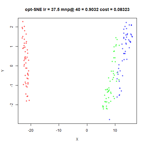
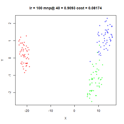
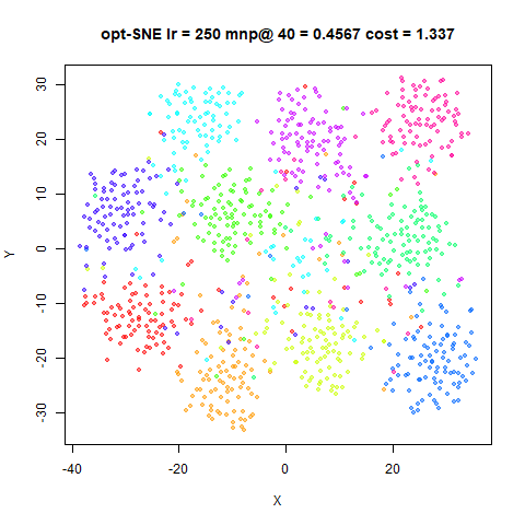
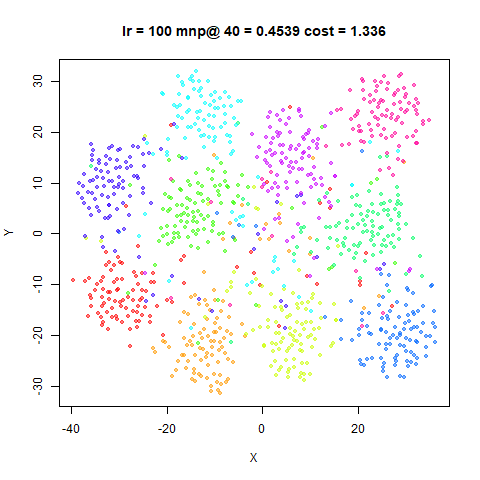
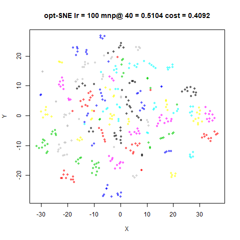
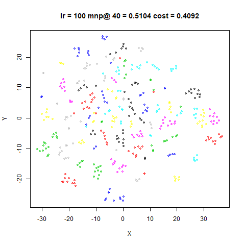
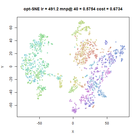
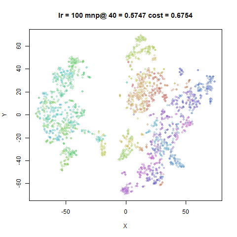
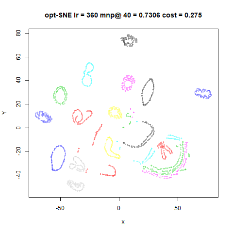
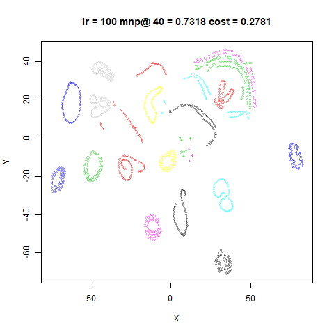
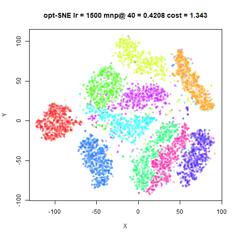
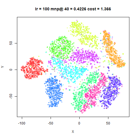
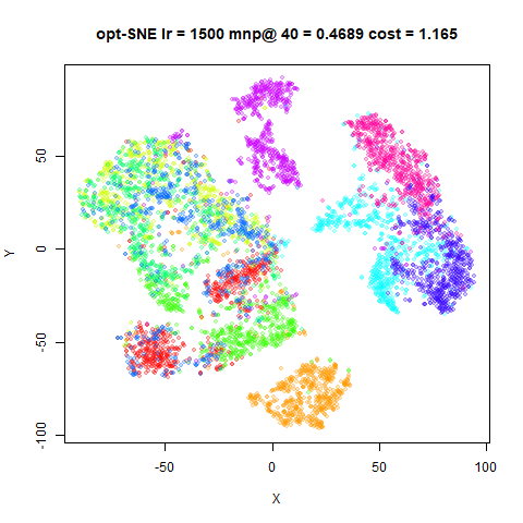
Left hand plots are those which use eta = "optsne". The resulting value of the learning rate is shown in the plot title. The right hand plots are for a fixed eta = 100.

iris

s1k

oli

frey

coil20

mnist6k

fashion6k

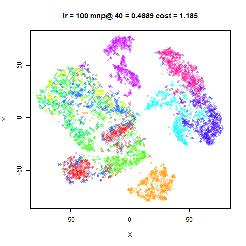Results are not very sensitive to the initial learning rate. oli shows no difference, because the opt-SNE settings choose eta = 100. iris and s1k divergences are slightly higher with eta = "optsne". For the other datasets, the divergences are all slightly lower, with the largest effect for the larger datasets, but even though the learning rate is an order of magnitude higher than the default for these datasets, the cost is less than 2% lower after 1000 iterations. The neighbor preservation values don’t show much difference either.

For the rest of the comparisons, we’ll use the eta = "optsne" results.

Early Exaggeration

As a reminder, Belkina and co-workers suggest examining the relative rate of change of the KL divergence during early exaggeration and terminating the exaggeration phase after the relative rate of change reaches a maximum.

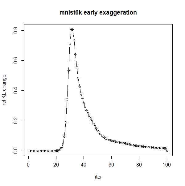
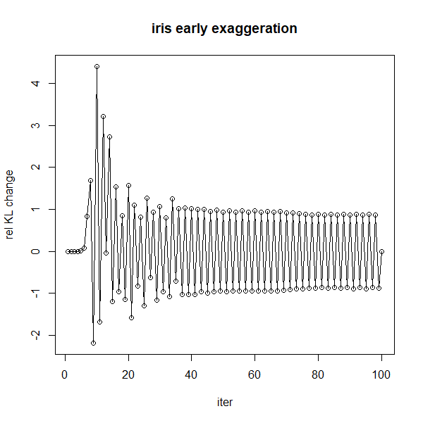
One objection to this is that it requires calculating the KL divergence at each iteration, which isn’t necessary during usual optimization. But there is an additional slight problem in that some datasets show quite noisy behavior during early exaggeration. Below is a plot of the relative KL change during early exaggeration for two datasets. On the left is mnist6k, which is quite well-behaved, and on the right, iris, which is not:

The mnist6k example uses a low learning rate of eta = 100 (much lower than then opt-SNE settings), and iris is using the eta = "optsne" setting which results in a fairly low learning rate of 37.5, but using eta = 100 doesn’t make a difference either and nor does reducing the momentum. The effect is substantially reduced by reducing the exaggeration_factor. Here are the results for exaggeration_factor = 2 and exaggeration_factor = 1.5:

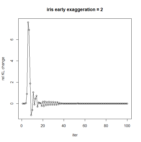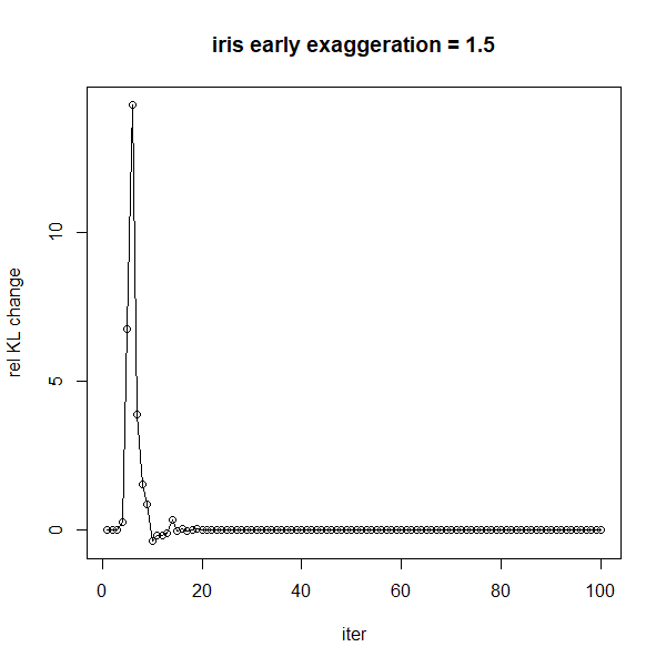I see a similar pattern with the typical standard t-SNE random layout. But at least for iris, the effect of early exaggeration doesn’t seem to do much to the final cost or layout. The noisy change in relative KL difference seems to be a fact of life for some datasets, and I saw similar patterns with oli.

At any rate it seems like these issues or something like them are also known to the authors, as the current (as of February 2019) implementation of opt-SNE is slightly more conservative in terminating the early exaggeration, as the procedure has been modified to:

• wait 15 iterations before monitoring the relative rate of change of KL.
• calculate the relative rate of change every three iterations, rather than every iteration.
• only terminate early exaggeration after the relative rate of change of KL has been observed to decrease three times.

Settings

The above is implemented in smallvis by specifying the ee_mon_epoch parameter. If specified, this value replaces that of epoch during early exaggeration, e.g. if ee_mon_epoch = 3 then the epoch code is run every 3 iterations, including running any callbacks and logging to console. The relative tolerance criterion is turned off, however, instead using the detection of the maximum of the rate of change. Additionally, the ee_mon_wait parameter controls how long to wait before checking the rate of change, and ee_mon_buffer specifies the number of times the rate of change check is passed but assumed to be a false positive due to noise. Setting ee_mon_buffer = 2 gives the default opt-SNE value, where early exaggeration is terminated only on the third occurrence.

iris_ee_tol <- smallvis(
  iris,
  perplexity = 40,
  eta = "optsne",
  Y_init = "spca",
  exaggeration_factor = 4,
  ee_mon_epoch = 3,
  ee_mon_wait = 15,
  ee_mon_buffer = 2
)

Results

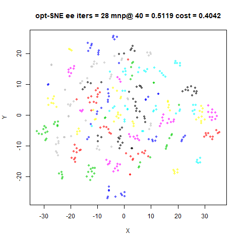
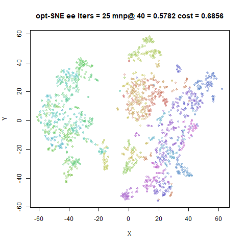
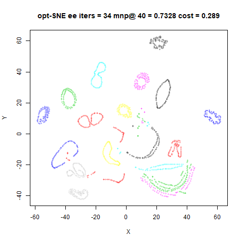
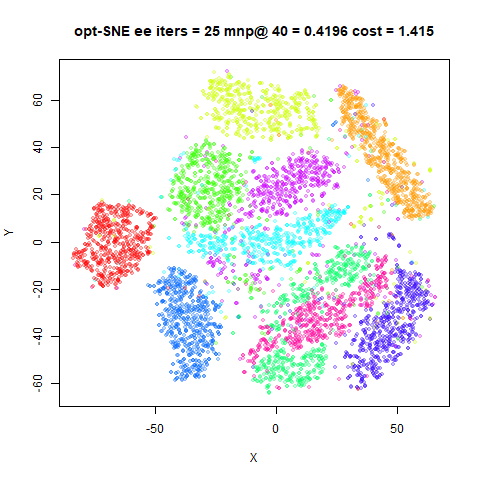
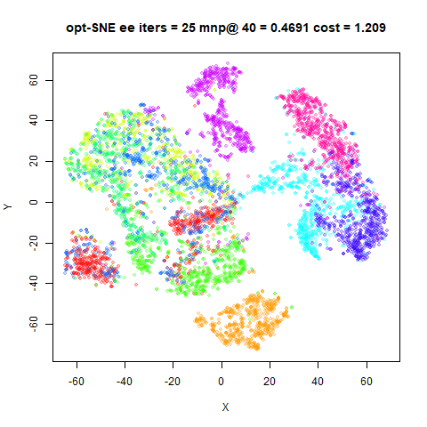
Left hand images are the results with the early exaggeration being monitored. The iteration at which the early exaggeration was stopped is given in the title of the image. The right hand images are the results from the previous section with eta = "optsne".

iris

s1k

oli

frey

coil20

mnist6k

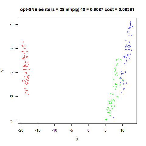
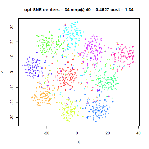
fashion6k

Rather than extending the exaggeration time, for all the datasets studied, the effect of the exaggeration monitoring is to terminate it much earlier than the full 100 iterations. No dataset uses exaggeration for more than 33 iterations.

Nonetheless, the results aren’t hugely affected. The final divergences are in general a little bit elevated, but there’s not a huge effect on either the neighbor preservation or the visual quality of the embedding. The mnist6k results are slightly different: the result with the ‘4’ cluster (in green at the bottom) is split by the ‘9’ cluster (magenta). This embedding turns up now and again with various t-SNE settings and seems to be nearly as stable as the un-split version in terms of KL divergence, but is obviously less appealing.

As early exaggeration is only 10% of the run time of the optimization, stopping after 30 iterations doesn’t save a huge amount of time, and doesn’t seem to help the embedding quality, at least if you initialize with scaled PCA.

Early stopping

Early stopping applies to the standard, un-exaggerated part of the optimization. Like with early exaggeration, the current implementation of opt-SNE slightly modifies the strategy given in the paper:

• waits 15 iterations before attempting to stop.
• checks every 5 iterations, rather than every iteration.
• the tolerance check is |\mathrm{KL}_{i-1} - \mathrm{KL}_{i}| / 5 < \mathrm{KL}_{i} / 5000, i.e. the relative tolerance check has been loosened from 1e-4 to 2e-4 (i.e. 1 / 5000). This can be changed by the user, but 5000 is the default.

This has been present in smallvis for a while, but by default the tolerance is set sufficiently low (1e-7) that you are unlikely to stop early with most datasets.

Settings

We’ll compare the tolerance used by the current version of opt-SNE, rather than the version given in the paper, but the difference won’t be too large. We’ll go back to 100 iterations of early exaggeration with no early stopping possible during that period of the optimization.

tol_wait = 15 sets the number of iterations to wait during standard optimization before allowing early stopping. In practice I don’t think I’ve seen any possibility of convergence occurring so early after turning off early exaggeration, but it’s included for completeness.

iris_early <- smallvis(
  iris,
  perplexity = 40,
  eta = "optsne",
  Y_init = "spca",
  exaggeration_factor = 4,
  epoch = 5,
  tol = 2e-4,
  tol_wait = 15
)

Results

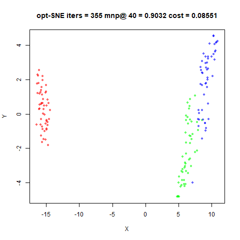
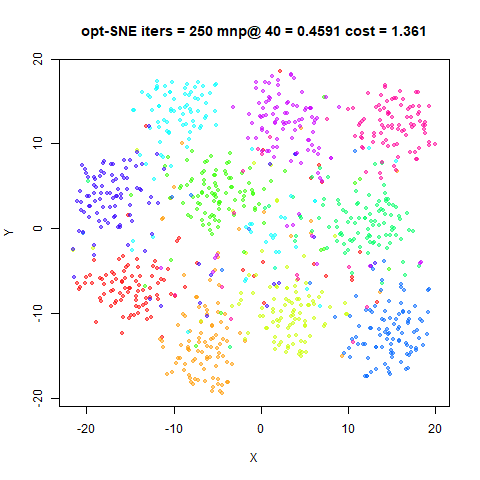
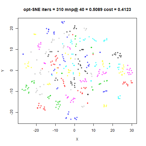
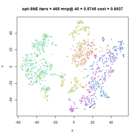
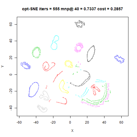
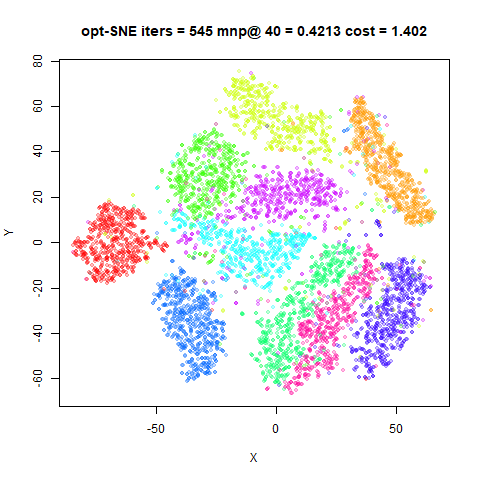
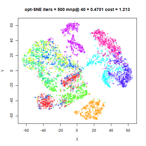
Early stopping results are on the left. The number of iterations used is given in the title. This includes the 100 iterations used in early embedding. The results on the right use all 1000 iterations.

iris

s1k

oli

frey

coil20

mnist6k

fashion6k

Early stopping definitely saves on iterations: no embedding runs for more than 555 iterations. And there’s no real difference to the neighbor preservation or the visual quality of the layouts. Possibly there are some local fine detail that’s different that isn’t readily visible from the images as shown. If you don’t care about that, then it seems like early stopping is a good idea.

Full opt-SNE

Finally, let’s put it all together: combining the dataset-dependent learning rate, early exaggeration monitoring and early stopping.

Settings

iris_optsne <- smallvis(
  iris,
  perplexity = 40,
  eta = "optsne",
  Y_init = "spca",
  exaggeration_factor = 4,
  ee_mon_epoch = 3,
  ee_mon_wait = 15,
  ee_mon_buffer = 2,
  epoch = 5,
  tol = 2e-4,
  tol_wait = 15
)

Results

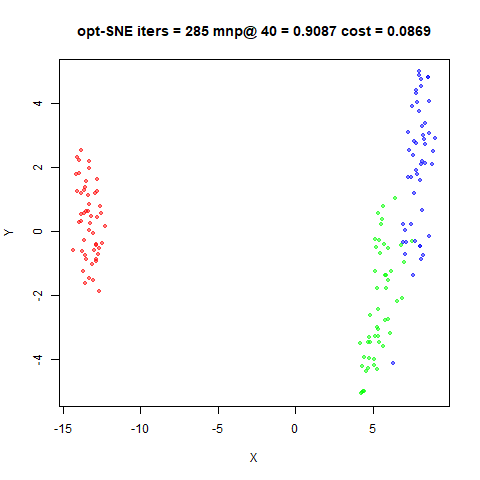
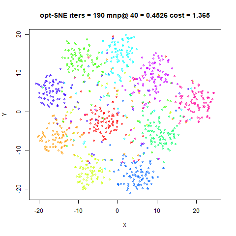
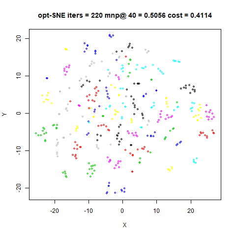
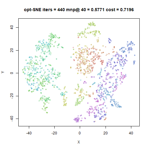
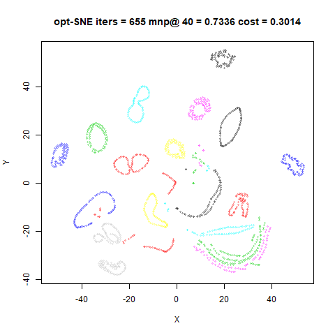
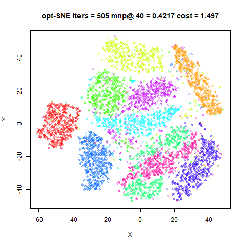
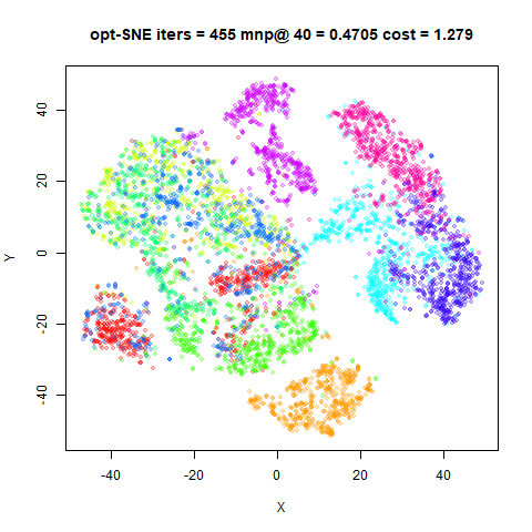
The full opt-SNE results are on the left. Again the total number of iterations is given in the title of the plot. The comparison on the right is from the previous section: full 100 iterations of early exaggeration and then early stopping.

iris

s1k

oli

frey

coil20

mnist6k

fashion6k

Combining the early exaggeration monitoring and the early stopping leads to even fewer iterations than just early stopping alone in all datasets except coil20, which takes an extra 100 iterations to stop.

Otherwise, these results are quite similar to the results from using only early stopping. The mnist6k results show the ‘4’ cluster split by the ‘9’ cluster, just as with the early exaggeration monitoring-only run.

Longer Epochs

Using the opt-SNE settings involves epochs of 3 and 5 iterations, which is much shorter than the smallvis default of 100, and even BH t-SNE normally only logs data every 50 iterations. If we use epoch = 50, can we get most of the speed up benefit of the opt-SNE settings? The main effect will be to prevent early stopping of the early exaggeration, but that doesn’t seem like a big problem, because the innovation of opt-SNE is to allow early exaggeration to go on for a lot longer than usual if needed, but for all the datasets looked at here, the only effect is to stop early exaggeration a lot earlier and it’s already a small fraction of the proportion of the number of iterations.

Settings

iris_epoch50 <- smallvis(
  iris,
  perplexity = 40,
  eta = "optsne",
  Y_init = "spca",
  exaggeration_factor = 4,
  epoch = 50,
  tol = 2e-4
)

Results

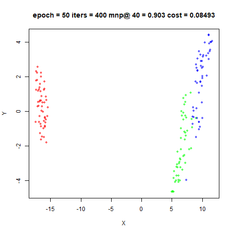
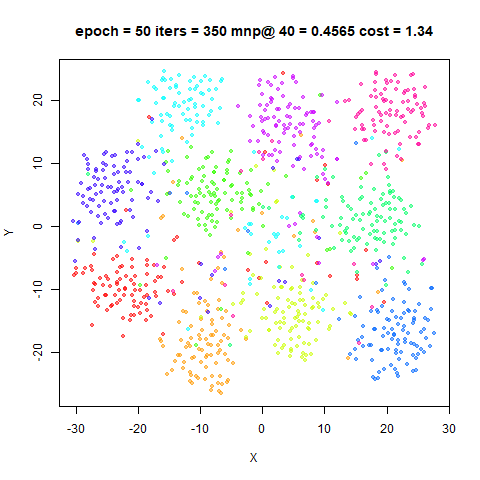
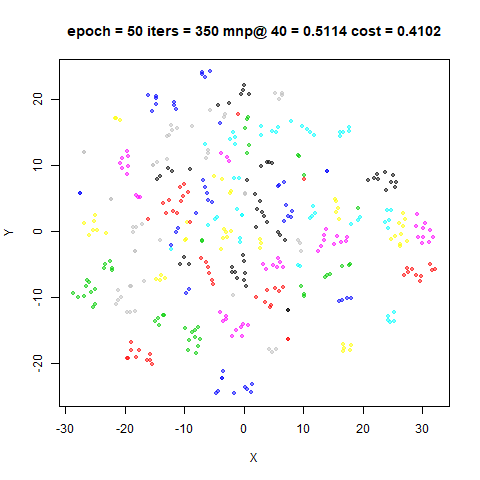
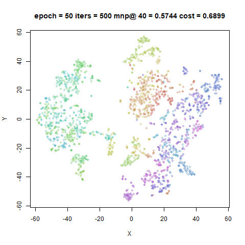
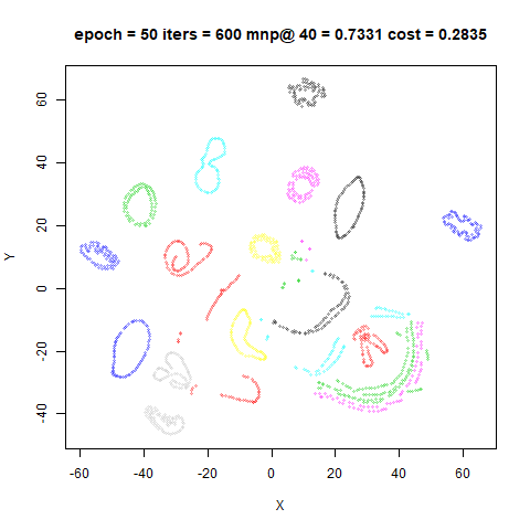
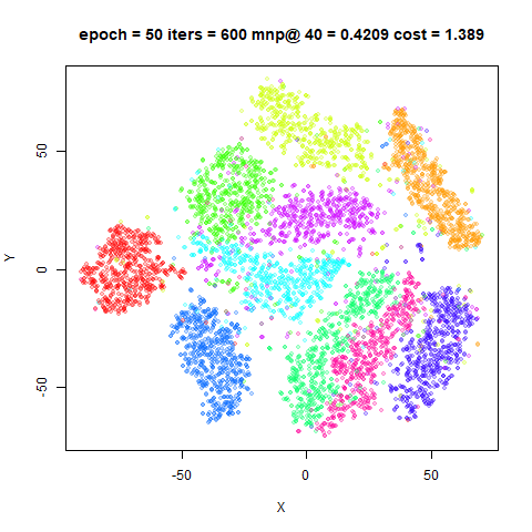
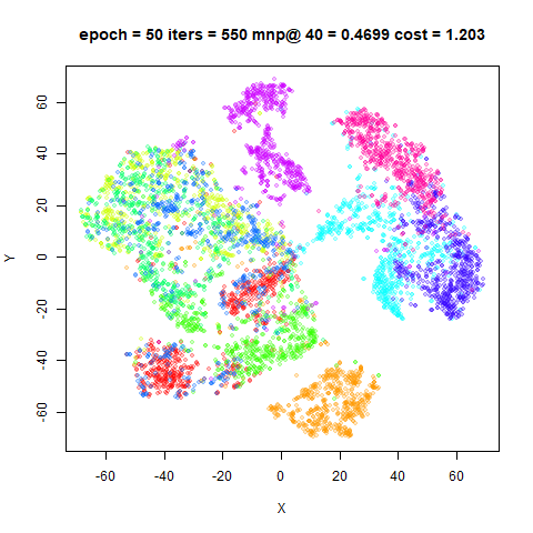
Results with using an epoch of 50 and no early exaggeration monitoring are shown on the left. The images on the right are of those from the early stopping results. The only difference between the two is that the images on the right used an epoch = 5, and therefore calculate the KL divergence and tolerance checks ten times more often.

iris

s1k

oli

frey

coil20

mnist6k

fashion6k

These results are very similar to each. By checking the tolerance less often we end up running for an extra 35-55 iterations, except for s1k which takes 100 more iterations.

It should be noted that there is a non-negligible cost to calculating the KL divergence more often. For mnist6k and fashion6k, setting epoch = 5 did increase the effective time per iteration by around 15%, even when the visualization callback was turned off. Obviously, the point at which this extra cost is worth it due to the optimization stopping earlier will depend on the speed of your hardware and the dataset size.

Conclusions

The opt-SNE settings are designed for very large datasets, so it’s perhaps not surprising that some of the recommendations don’t have a big effect for the small datasets that smallvis can handle.

Setting eta = "optsne" seems mildly helpful for larger datasets. It may give a learning rate that’s too low for small datasets, however.

The early exaggeration monitoring wasn’t that helpful for the datasets studied here: it reduced the time spent in early exaggeration, but it wasn’t that long to begin with. None of the datasets tested here indicated that more time in early exaggeration than 100 iterations was needed, so you may as well leave it at that default.

Early stopping via the tol setting is definitely helpful. With the opt-SNE setting of tol = 2e-4, all of the tested datasets had converged by iteration 600 at the latest, rather than terminating at the default of 1000. Using the opt-SNE epoch settings of 3 (for early exaggeration) and 5 does seem excessive, though. Probably a setting of between 25-50 is a better trade off between early stopping opportunity and KL divergence calculation time.

Up: Documentation Home.