g-SNE

This article retains its original experiments and examples. For current package usage, see the usage guide.

The g-SNE paper (with matlab code on github) suggests a modification of t-SNE to add a second divergence that is more focused on matching similarities due to longer distances. The idea is that a weighted combination of the two will balance global and local structure.

The g-SNE cost function is:

C = \sum_{ij} p_{ij} \log \frac{p_{ij}}{q_{ij}} + \lambda \sum_{ij} \hat{p}_{ij} \log \frac{\hat{p}_{ij}}{\hat{q}_{ij}}

with \lambda being a weighting factor as in NeRV, the un-hatted part of the cost function being the same as t-SNE, and the hatted quantities referring to using the reciprocal of the usual t-SNE kernel:

\hat{w}_{ij} = 1 + d_{ij}^2 = \frac{1}{w_{ij}}

The gradient is:

\frac{\partial C}{\partial \mathbf{y}_i} = 4 \sum_j \left[ \left(p_{ij} - q_{ij}\right) -\lambda \left( \hat{p}_{ij} - \hat{q}_{ij} \right) \right]w_{ij} \left( \mathbf{y}_i - \mathbf{y}_j \right)

As was also apparent from the cost function, you can see that this reduces back to t-SNE when \lambda = 0.

Datasets

See the Datasets page.

Settings

To use g-SNE in smallvis, use method = "gsne", which uses a default \lambda = 1, which is used in most of the datasets in the paper. Different values of \lambda can be specified by using e.g. method = list("gsne", lambda = 5). In the g-SNE paper, values of lambda between 0 and 10 are considered, so we will look at 1, 2.5, 5 and 10.

Other settings will be kept standard. The word ‘perplexity’ doesn’t seem to appear in the paper at all, and the github code examples use the default value of 30, so perplexity = 40 is going to be fine here.

Early exaggeration also isn’t mentioned in the paper, and in my experiments it made no difference to the results, but it’s on by default in the code on github, so I’ve also used it to here. The exaggeration is not applied to \hat{P} in either smallvis or the matlab implementation.

iris_gsne <- smallvis(
  iris,
  method = list("gsne", lambda = 5),
  perplexity = 40,
  eta = 100,
  Y_init = "spca",
  exaggeration_factor = 4
)

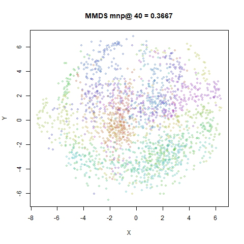
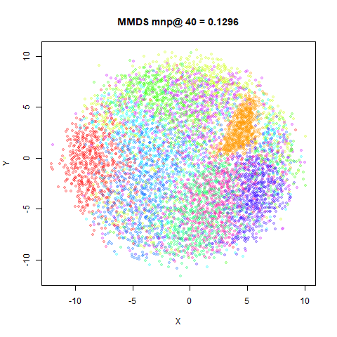
An obvious point of comparison is t-SNE, which is the same as g-SNE with \lambda = 0. For preserving global distances, we can use metric MDS. We’ve looked at MMDS elsewhere, but in this case we will use the t-SNE scaling (not that it makes much difference).

iris_tsne <- smallvis(
  iris,
  perplexity = 40,
  eta = 100,
  Y_init = "spca",
  exaggeration_factor = 4
)
iris_mmds <- smallvis(
  iris,
  eta = 1e-5,
  max_iter = 2000,
  Y_init = "spca",
  method = "mmds"
)

Results

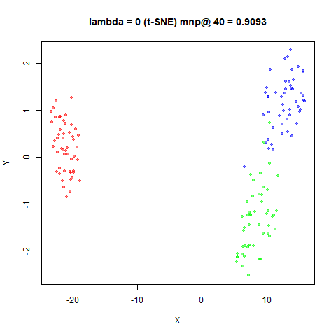
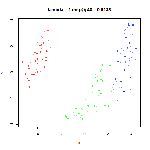
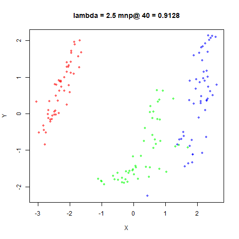
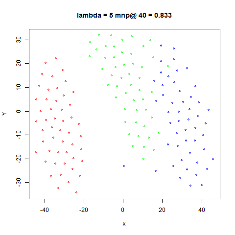
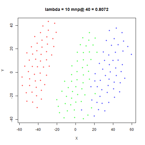
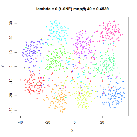
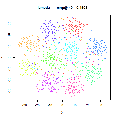
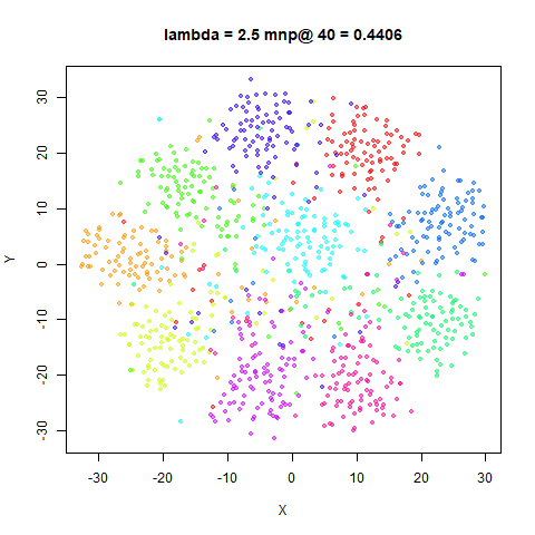
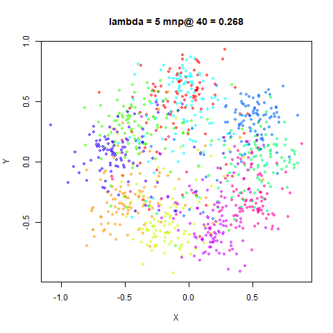
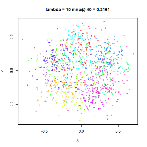
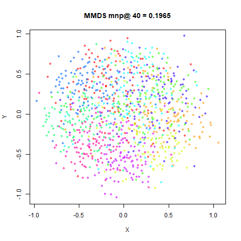
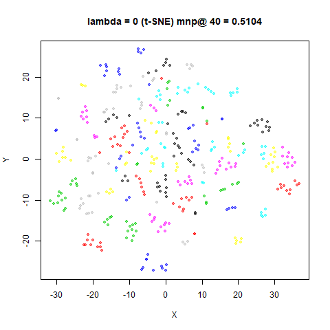
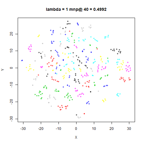
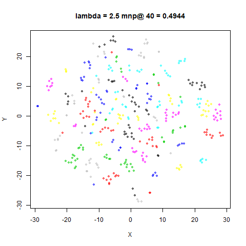
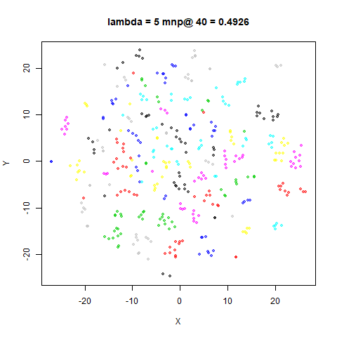
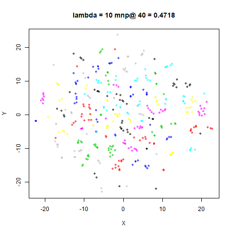
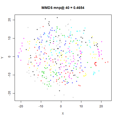
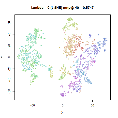
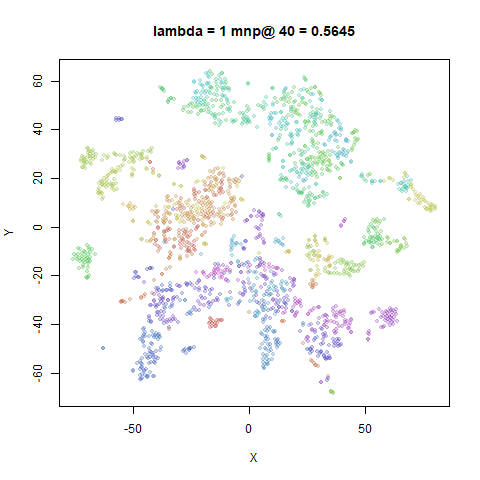
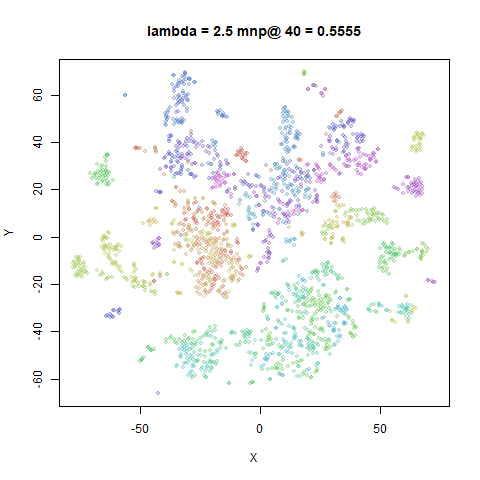
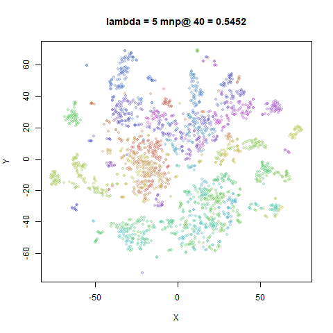
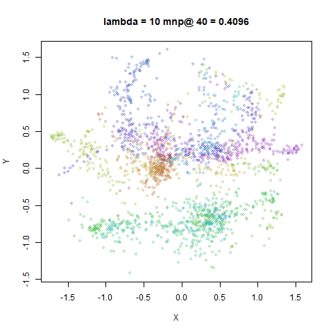
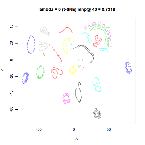
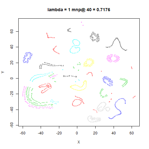
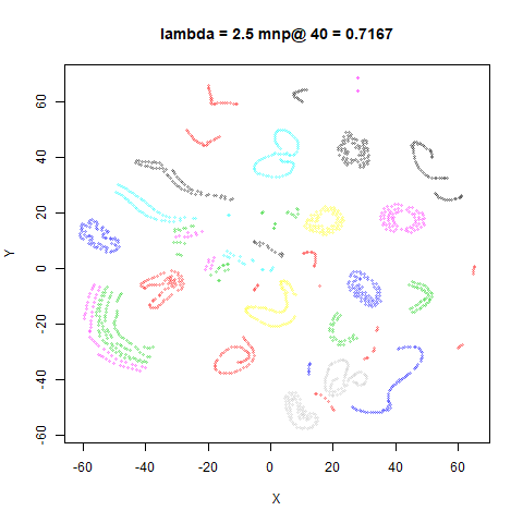
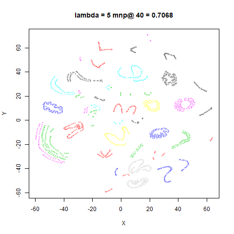
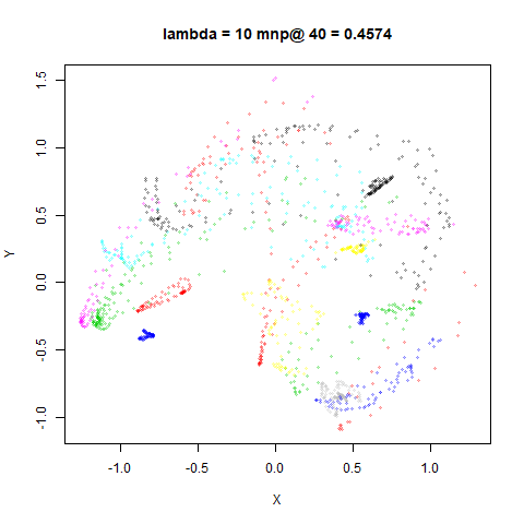
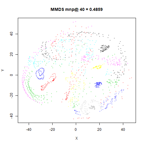
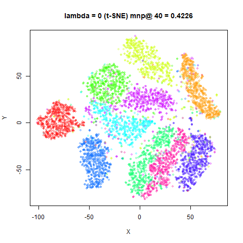
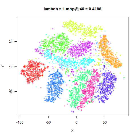
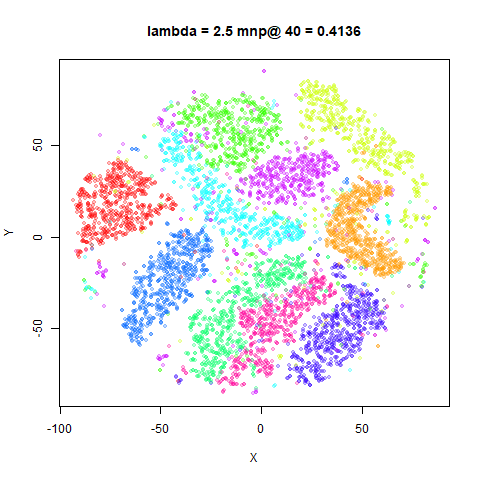
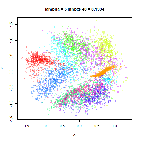
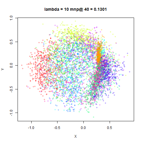
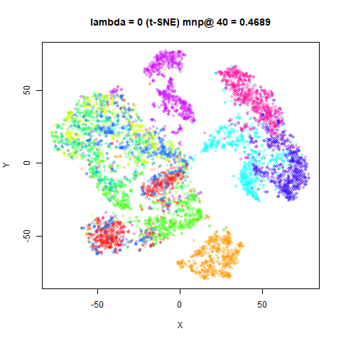
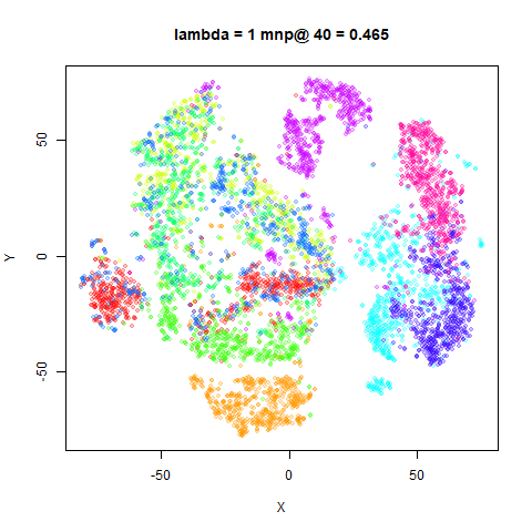
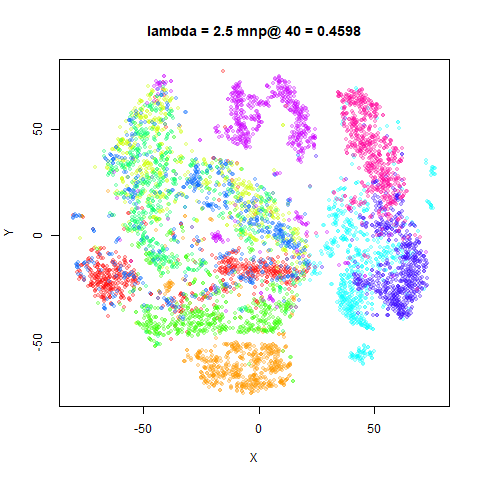
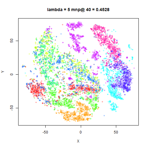
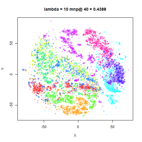
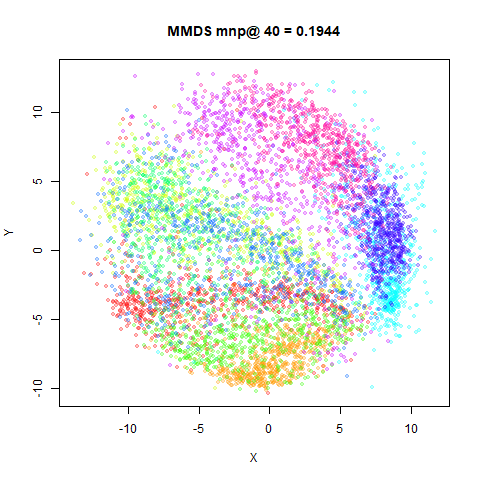
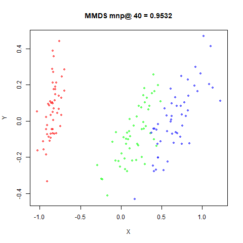
For each dataset, from left-to-right and top-to-bottom, lambda increased from 0 (t-SNE) to 1, 2.5, 5 and 10. The bottom right image is MMDS.

iris

s1k

oli

frey

coil20

mnist6k

fashion6k

Conclusions

Except for iris, it’s clear that, in general, increasing \lambda makes the g-SNE progressively approach the sort of layout we’d expect with MMDS. I’m just not sure that I particularly like any of the intermediate results more than just sticking with the t-SNE results. I think starting from the scaled PCA initialization gives you a lot of the global layout you would want. lambda values between 1 and 2.5 seem the best place to start exploring.

On the other hand, the authors use a topological clique analysis involving Betti numbers for some gene expression data and conclude that the g-SNE plot represents the data better. Unfortunately, the plots are rather small, and for a second example which required a value lambda = 5 for optimal results, the plots aren’t shown.

February 28, 2019