Barnes-Hut and native acceleration

Most smallvis methods calculate interactions between every pair of observations. That makes them convenient for experimentation on small datasets, but their time and memory requirements grow quadratically. For larger datasets, t-SNE, SSNE, HSSNE, dynamic HSSNE, SNeRV, t-distributed elastic embedding (TEE), LargeVis, UMAP, t-UMAP, Jensen-Shannon SNE, Hellinger SNE, and chi-squared SNE can combine sparse neighbor affinities with Barnes-Hut repulsion.

Run Barnes-Hut t-SNE

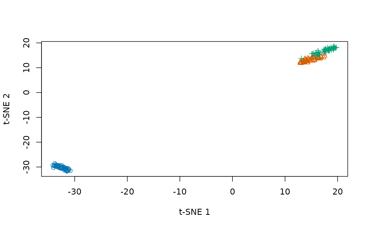
This configuration uses approximate nearest neighbors, a sparse neighbor graph, and two native workers. Iris is small enough to run as a quick example; the configuration becomes useful when the dense calculation is too expensive.

set.seed(42)
bh_fit <- smallvis(
  iris,
  method = "tsne",
  bh = TRUE,
  inp_kernel = "knn",
  nn = "approximate",
  n_threads = 2,
  perplexity = 30,
  exaggeration_factor = 12,
  stop_lying_iter = 250,
  Y_init = "spca",
  epoch_callback = FALSE,
  verbose = FALSE
)
species <- as.integer(iris$Species)
plot(
  bh_fit,
  col = c("#0072B2", "#D55E00", "#009E73")[species],
  pch = species,
  xlab = "t-SNE 1",
  ylab = "t-SNE 2"
)

Barnes-Hut requires two output dimensions. The default is theta = 0.5. Smaller values open more cells and require more work. Zero evaluates the repulsive sum exactly for the chosen input graph.

The example uses binary k-nearest-neighbor affinities. Use inp_kernel = "nngaussian" for Gaussian perplexity calibration over neighbors instead. The input kernel and Barnes-Hut arguments describe these controls.

You can also use method = list("hssne", alpha = 0.5) or method = list("tee", lambda = 0.01) with "knn" or "nngaussian" affinities. HSSNE changes the tail of the output kernel, and method = "dhssne" allows alpha to change at each epoch. TEE keeps the t-SNE kernel and uses a fixed repulsion multiplier. The same input kernels work with method = "ssne", method = "snerv", method = "largevis", method = "tumap", method = "jssne", method = "hlsne", and method = "chsne".

If you already have a neighbor graph, pass its idx and dist matrices in a list as neighbors = graph and leave nn unset. This works for dense and Barnes-Hut methods using "knn", "nngaussian", or "skd" affinities. With "nngaussian", a perplexity of 30 takes 90 non-self neighbors per row on a dataset with at least 91 observations. UMAP uses smooth kNN affinities (inp_kernel = "skd"), which are also available for t-UMAP. With perplexity = 30, "skd" takes 29 non-self neighbors per row. The saved graph supplies the affinities, so you can leave pca = FALSE and let Y_init = "spca" compute the starting coordinates.

Accelerate a dense calculation

For dense t-SNE, use_cpp = TRUE enables native calibration and gradient calculations. It retains the dense pairwise representation, so this speeds up a calculation without removing its quadratic memory requirement:

native_fit <- smallvis(
  iris,
  Y_init = "spca",
  perplexity = 30,
  use_cpp = TRUE,
  n_threads = 2,
  epoch_callback = FALSE,
  verbose = FALSE
)
dim(native_fit)

## [1] 150   2

Native acceleration covers selected calculations and methods. The specialized dense gradient kernels use two output dimensions; other dimensions use the general R calculations for those steps. use_cpp = TRUE therefore does not imply that every stage or every method runs in C++.

Choose a thread count

n_threads = 0 selects serial execution. Positive values control native worker threads in the supported stages, including neighbor search. More workers can help larger inputs, but setup costs, memory bandwidth, and work still performed in R limit the improvement. Numerical libraries can also have their own thread settings.

Start with a modest worker count and measure the complete call on your data. Changing from dense affinities to a sparse neighbor graph also changes the input problem, so compare those embeddings as different approximations rather than interpreting the runtime alone.